Domain decomposition methods
In mathematics, numerical analysis, and numerical partial differential equations, domain decomposition methods solve a boundary value problem by splitting it into smaller boundary value problems on subdomains and iterating to coordinate the solution between adjacent subdomains. A coarse problem with one or few unknowns per subdomain is used to further coordinate the solution between the subdomains globally. The problems on the subdomains are independent, which makes domain decomposition methods suitable for parallel computing. Domain decomposition methods are typically used as preconditioners for Krylov space iterative methods, such as the conjugate gradient method, GMRES, and LOBPCG.
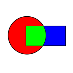
In overlapping domain decomposition methods, the subdomains overlap by more than the interface. Overlapping domain decomposition methods include the Schwarz alternating method and the additive Schwarz method. Many domain decomposition methods can be written and analyzed as a special case of the abstract additive Schwarz method.
In non-overlapping methods, the subdomains intersect only on their interface. In primal methods, such as Balancing domain decomposition and BDDC, the continuity of the solution across subdomain interface is enforced by representing the value of the solution on all neighboring subdomains by the same unknown. In dual methods, such as FETI, the continuity of the solution across the subdomain interface is enforced by Lagrange multipliers. The FETI-DP method is hybrid between a dual and a primal method.
Non-overlapping domain decomposition methods are also called iterative substructuring methods.
Mortar methods are discretization methods for partial differential equations, which use separate discretization on nonoverlapping subdomains. The meshes on the subdomains do not match on the interface, and the equality of the solution is enforced by Lagrange multipliers, judiciously chosen to preserve the accuracy of the solution. In the engineering practice in the finite element method, continuity of solutions between non-matching subdomains is implemented by multiple-point constraints.
Finite element simulations of moderate size models require solving linear systems with millions of unknowns. Several hours per time step is an average sequential run time, therefore, parallel computing is a necessity. Domain decomposition methods embody large potential for a parallelization of the finite element methods, and serve a basis for distributed, parallel computations.
Example 1: 1D Linear BVP
[math]\displaystyle{ u''(x)-u(x)=0 }[/math]
[math]\displaystyle{ u(0)=0, u(1)=1 }[/math]
The exact solution is:
[math]\displaystyle{ u(x)=\frac{e^x-e^{-x}}{e^{1}-e^{-1}} }[/math]
Subdivide the domain into two subdomains, one from [math]\displaystyle{ \left[0,\frac{1}{2}\right] }[/math] and another from [math]\displaystyle{ \left[\frac{1}{2},1\right] }[/math]. In the left subdomain define the interpolating function [math]\displaystyle{ v_1(x) }[/math] and in the right define [math]\displaystyle{ v_2 (x) }[/math]. At the interface between these two subdomains the following interface conditions shall be imposed:
[math]\displaystyle{ v_1\left(\frac{1}{2}\right)=v_2 \left(\frac{1}{2}\right) }[/math]
[math]\displaystyle{ v_1'\left(\frac{1}{2}\right)=v_2'\left(\frac{1}{2}\right) }[/math]
Let the interpolating functions be defined as:
[math]\displaystyle{ v_1 (x) =\sum_{n=0}^{N} u_{n} T_n (y_1(x)) }[/math]
[math]\displaystyle{ v_2 (x) =\sum_{n=0}^{N} u_{n+N} T_n (y_2(x)) }[/math]
[math]\displaystyle{ y_1(x)=4x-1 }[/math]
[math]\displaystyle{ y_2(x)=4x-3 }[/math]
Where [math]\displaystyle{ T_n (y) }[/math] is the nth cardinal function of the chebyshev polynomials of the first kind with input argument y.
If N=4 then the following approximation is obtained by this scheme:
[math]\displaystyle{ u_1 =0.06236 }[/math]
[math]\displaystyle{ u_2 =0.21495 }[/math]
[math]\displaystyle{ u_3 =0.37428 }[/math]
[math]\displaystyle{ u_4 =0.44341 }[/math]
[math]\displaystyle{ u_5 =0.51492 }[/math]
[math]\displaystyle{ u_6 =0.69972 }[/math]
[math]\displaystyle{ u_7 =0.90645 }[/math]
This was obtained with the following MATLAB code.
clear all
N = 4;
a1 = 0; b1 = 1/2;

[T D1 D2 E1 E2 x xsub] = cheb(N,a1,b1); % the diff matrices on [0,1/2] are the same
%as those on [1/2 1].
I = eye(N+1);
H = D2-I;
H1 = 1 zeros(1,N)]; H(2:end-1,:); [zeros(1,N) 1;
H1 = [H1 [zeros(N,N+1); -[1 zeros(1,N)]]];
H2 = [D1(1,:); H(2:end-1,:); [zeros(1,N) 1]];
H2 = [[-D1(N+1,:); zeros(N,N+1)] H2];
K = [H1; H2];
F = [zeros(2*N+1,1); 1];
u = K\F;
xx = -cos(pi*(0:N)'/N);
x1 = 1/4*(xx+1); x2 = 1/4*(xx+3);
x = [x1; x2];
uex = (exp(x)-exp(-x))./(exp(1)-exp(-1));
See also
External links
- The official Domain Decomposition Methods page
- "Domain Decomposition - Numerical Simulations page". http://www.domain-decomposition.com/.
 |


