Finite difference method
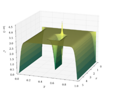
| Differential equations |
|---|
 |
| Classification |
| Solution |
In numerical analysis, finite-difference methods (FDM) are a class of numerical techniques for solving differential equations by approximating derivatives with finite differences. Both the spatial domain and time domain (if applicable) are discretized, or broken into a finite number of intervals, and the values of the solution at the end points of the intervals are approximated by solving algebraic equations containing finite differences and values from nearby points.
Finite difference methods convert ordinary differential equations (ODE) or partial differential equations (PDE), which may be nonlinear, into a system of linear equations that can be solved by matrix algebra techniques. Modern computers can perform these linear algebra computations efficiently, and this, along with their relative ease of implementation, has led to the widespread use of FDM in modern numerical analysis.[1] Today, FDMs are one of the most common approaches to the numerical solution of PDE, along with finite element methods.[1]
Derive difference quotient from Taylor's polynomial
For a n-times differentiable function, by Taylor's theorem the Taylor series expansion is given as
Where n! denotes the factorial of n, and Rn(x) is a remainder term, denoting the difference between the Taylor polynomial of degree n and the original function.
Following is the process to derive an approximation for the first derivative of the function f by first truncating the Taylor polynomial plus remainder: Dividing across by h gives: Solving for :
Assuming that is sufficiently small, the approximation of the first derivative of f is:
This is similar to the definition of derivative, which is: except for the limit towards zero (the method is named after this).
Accuracy and order
The error in a method's solution is defined as the difference between the approximation and the exact analytical solution. The two sources of error in finite difference methods are round-off error, the loss of precision due to computer rounding of decimal quantities, and truncation error or discretization error, the difference between the exact solution of the original differential equation and the exact quantity assuming perfect arithmetic (no round-off).
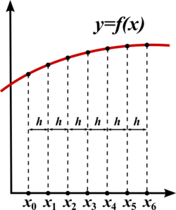
To use a finite difference method to approximate the solution to a problem, one must first discretize the problem's domain. This is usually done by dividing the domain into a uniform grid (see image). This means that finite-difference methods produce sets of discrete numerical approximations to the derivative, often in a "time-stepping" manner.
An expression of general interest is the local truncation error of a method. Typically expressed using Big-O notation, local truncation error refers to the error from a single application of a method. That is, it is the quantity if refers to the exact value and to the numerical approximation. The remainder term of the Taylor polynomial can be used to analyze local truncation error. Using the Lagrange form of the remainder from the Taylor polynomial for , which is the dominant term of the local truncation error can be discovered. For example, again using the forward-difference formula for the first derivative, knowing that , and with some algebraic manipulation, this leads to and further noting that the quantity on the left is the approximation from the finite difference method and that the quantity on the right is the exact quantity of interest plus a remainder, clearly that remainder is the local truncation error. A final expression of this example and its order is:
In this case, the local truncation error is proportional to the step sizes. The quality and duration of simulated FDM solution depends on the discretization equation selection and the step sizes (time and space steps). The data quality and simulation duration increase significantly with smaller step size.[2] Therefore, a reasonable balance between data quality and simulation duration is necessary for practical usage. Large time steps are useful for increasing simulation speed in practice. However, time steps which are too large may create instabilities and affect the data quality.[3][4]
The von Neumann and Courant-Friedrichs-Lewy criteria are often evaluated to determine the numerical model stability.[3][4][5][6]
Example: ordinary differential equation
For example, consider the ordinary differential equation The Euler method for solving this equation uses the finite difference quotient to approximate the differential equation by first substituting it for then applying a little algebra (multiplying both sides by h, and then adding to both sides) to get The last equation is a finite-difference equation, and solving this equation gives an approximate solution to the differential equation.
Example: The heat equation
Consider the normalized heat equation in one dimension, with homogeneous Dirichlet boundary conditions
One way to numerically solve this equation is to approximate all the derivatives by finite differences. First partition the domain in space using a mesh and in time using a mesh . Assume a uniform partition both in space and in time, so the difference between two consecutive space points will be h and between two consecutive time points will be k. The points
will represent the numerical approximation of
Explicit method
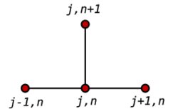
Using a forward difference at time and a second-order central difference for the space derivative at position (FTCS) gives the recurrence equation:
This is an explicit method for solving the one-dimensional heat equation.
One can obtain from the other values this way:
where
So, with this recurrence relation, and knowing the values at time n, one can obtain the corresponding values at time n+1. and must be replaced by the boundary conditions, in this example they are both 0.
This explicit method is known to be numerically stable and convergent whenever .[7] The numerical errors are proportional to the time step and the square of the space step:
Implicit method

Using the backward difference at time and a second-order central difference for the space derivative at position (The Backward Time, Centered Space Method "BTCS") gives the recurrence equation:
This is an implicit method for solving the one-dimensional heat equation.
One can obtain from solving a system of linear equations:
The scheme is always numerically stable and convergent but usually more numerically intensive than the explicit method as it requires solving a system of numerical equations on each time step. The errors are linear over the time step and quadratic over the space step:
Crank–Nicolson method
Finally, using the central difference at time and a second-order central difference for the space derivative at position ("CTCS") gives the recurrence equation:
This formula is known as the Crank–Nicolson method.
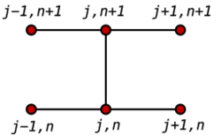
One can obtain from solving a system of linear equations:
The scheme is always numerically stable and convergent but usually more numerically intensive as it requires solving a system of numerical equations on each time step. The errors are quadratic over both the time step and the space step:
Comparison
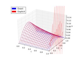
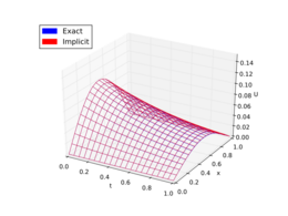
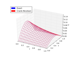
To summarize, usually the Crank–Nicolson scheme is the most accurate scheme for small time steps. For larger time steps, the implicit scheme works better since it is less computationally demanding. The explicit scheme is the least accurate and can be unstable, but is also the easiest to implement and the least numerically intensive.
Here is an example. The figures below present the solutions given by the above methods to approximate the heat equation
with the boundary condition
The exact solution is
Example: The Laplace operator
The (continuous) Laplace operator in -dimensions is given by . The discrete Laplace operator depends on the dimension .
In 1D the Laplace operator is approximated as This approximation is usually expressed via the following stencil and which represents a symmetric, tridiagonal matrix. For an equidistant grid one gets a Toeplitz matrix.
The 2D case shows all the characteristics of the more general n-dimensional case. Each second partial derivative needs to be approximated similar to the 1D case which is usually given by the following stencil
Consistency
Consistency of the above-mentioned approximation can be shown for highly regular functions, such as . The statement is
To prove this, one needs to substitute Taylor Series expansions up to order 3 into the discrete Laplace operator.
Properties
Subharmonic
Similar to continuous subharmonic functions one can define subharmonic functions for finite-difference approximations
Mean value
One can define a general stencil of positive type via
If is (discrete) subharmonic then the following mean value property holds where the approximation is evaluated on points of the grid, and the stencil is assumed to be of positive type.
A similar mean value property also holds for the continuous case.
Maximum principle
For a (discrete) subharmonic function the following holds where are discretizations of the continuous domain , respectively the boundary .
A similar maximum principle also holds for the continuous case.
The SBP-SAT method
The SBP-SAT (summation by parts - simultaneous approximation term) method is a stable and accurate technique for discretizing and imposing boundary conditions of a well-posed linear partial differential equation using high order finite differences.[8][9]
The method is based on finite differences where the differentiation operators exhibit summation-by-parts properties. Typically, these operators consist of differentiation matrices with central difference stencils in the interior with carefully chosen one-sided boundary stencils designed to mimic integration-by-parts in the discrete setting. Using the SAT technique, the boundary conditions of the PDE are imposed weakly, where the boundary values are "pulled" towards the desired conditions rather than exactly fulfilled. If the tuning parameters (inherent to the SAT technique) are chosen properly, the resulting system of ODE's will exhibit similar energy behavior as the continuous PDE, i.e. the system has no non-physical energy growth. This guarantees stability if an integration scheme with a stability region that includes parts of the imaginary axis, such as the fourth order Runge-Kutta method, is used. This makes the SAT technique an attractive method of imposing boundary conditions for higher order finite difference methods, in contrast to for example the injection method, which typically will not be stable if high order differentiation operators are used.
See also
- Finite element method
- Finite difference
- Finite difference time domain
- Infinite difference method
- Stencil (numerical analysis)
- Finite difference coefficients
- Five-point stencil
- Lax–Richtmyer theorem
- Finite difference methods for option pricing
- Upwind differencing scheme for convection
- Central differencing scheme
- Discrete Poisson equation
- Discrete Laplace operator
References
- ↑ 1.0 1.1 Christian Grossmann; Hans-G. Roos; Martin Stynes (2007). Numerical Treatment of Partial Differential Equations. Springer Science & Business Media. p. 23. ISBN 978-3-540-71584-9. https://archive.org/details/numericaltreatme00gros_820.
- ↑ Arieh Iserles (2008). A first course in the numerical analysis of differential equations. Cambridge University Press. p. 23. ISBN 9780521734905. https://archive.org/details/firstcoursenumer00iser.
- ↑ 3.0 3.1 Hoffman JD; Frankel S (2001). Numerical methods for engineers and scientists. CRC Press, Boca Raton.
- ↑ 4.0 4.1 Jaluria Y; Atluri S (1994). "Computational heat transfer". Computational Mechanics 14 (5): 385–386. doi:10.1007/BF00377593. Bibcode: 1994CompM..14..385J.
- ↑ Majumdar P (2005). Computational methods for heat and mass transfer (1st ed.). Taylor and Francis, New York.
- ↑ Smith GD (1985). Numerical solution of partial differential equations: finite difference methods (3rd ed.). Oxford University Press.
- ↑ Crank, J. The Mathematics of Diffusion. 2nd Edition, Oxford, 1975, p. 143.
- ↑ Bo Strand (1994). "Summation by Parts for Finite Difference Approximations for d/dx". Journal of Computational Physics 110 (1): 47–67. doi:10.1006/jcph.1994.1005. Bibcode: 1994JCoPh.110...47S.
- ↑ Mark H. Carpenter; David I. Gottlieb; Saul S. Abarbanel (1994). "Time-stable boundary conditions for finite-difference schemes solving hyperbolic systems: Methodology and application to high-order compact schemes". Journal of Computational Physics 111 (2): 220–236. doi:10.1006/jcph.1994.1057. Bibcode: 1994JCoPh.111..220C.
Further reading
- K.W. Morton and D.F. Mayers, Numerical Solution of Partial Differential Equations, An Introduction. Cambridge University Press, 2005.
- Autar Kaw and E. Eric Kalu, Numerical Methods with Applications, (2008) [1]. Contains a brief, engineering-oriented introduction to FDM (for ODEs) in Chapter 08.07.
- John Strikwerda (2004). Finite Difference Schemes and Partial Differential Equations (2nd ed.). SIAM. ISBN 978-0-89871-639-9.
- Smith, G. D. (1985), Numerical Solution of Partial Differential Equations: Finite Difference Methods, 3rd ed., Oxford University Press
- Peter Olver (2013). Introduction to Partial Differential Equations. Springer. Chapter 5: Finite differences. ISBN 978-3-319-02099-0. http://www.math.umn.edu/~olver/pde.html..
- Randall J. LeVeque, Finite Difference Methods for Ordinary and Partial Differential Equations, SIAM, 2007.
- Sergey Lemeshevsky, Piotr Matus, Dmitriy Poliakov(Eds): "Exact Finite-Difference Schemes", De Gruyter (2016). DOI: https://doi.org/10.1515/9783110491326 .
- Mikhail Shashkov: Conservative Finite-Difference Methods on General Grids, CRC Press, ISBN 0-8493-7375-1 (1996).
 |
