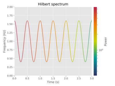
Hilbert spectrum
The Hilbert spectrum (sometimes referred to as the Hilbert amplitude spectrum), named after David Hilbert, is a statistical tool that can help in distinguishing among a mixture of moving signals. The spectrum itself is decomposed into its component sources using independent component analysis. The separation of the combined effects of unidentified sources (blind signal separation) has applications in climatology, seismology, and biomedical imaging.
Conceptual summary
The Hilbert spectrum is computed by way of a 2-step process consisting of:
- Preprocessing a signal separate it into intrinsic mode functions using a mathematical decomposition such as singular value decomposition (SVD) or empirical mode decomposition (EMD);
- Applying the Hilbert transform to the results of the above step to obtain the instantaneous frequency spectrum of each of the components.
The Hilbert transform defines the imaginary part of the function to make it an analytic function (sometimes referred to as a progressive function), i.e. a function whose signal strength is zero for all frequency components less than zero.
With the Hilbert transform, the singular vectors give instantaneous frequencies that are functions of time, so that the result is an energy distribution over time and frequency.
The result is an ability to capture time-frequency localization to make the concept of instantaneous frequency and time relevant (the concept of instantaneous frequency is otherwise abstract or difficult to define for all but monocomponent signals).
Definition
For a given signal [math]\displaystyle{ x(t) }[/math] decomposed (with for example Empirical Mode Decomposition) to
[math]\displaystyle{ x(t) = r(t) + \sum_{j=1}^{k} c_j(t) }[/math]
where [math]\displaystyle{ k }[/math] is the number of intrinsic mode functions that [math]\displaystyle{ x(t) }[/math] consists of and
[math]\displaystyle{ c_j(t) = \mathbb{R}\big\{ a_j(t) e^{-i\theta_j(t)} \big\} = a_j(t) \cos\big(\theta_j(t)\big) }[/math]
The instantaneous angle frequency is then defined as
[math]\displaystyle{ \omega_j(t) = \frac{d\theta_j(t)}{dt} }[/math]
From this, we can define the Hilbert Spectrum[1] for [math]\displaystyle{ c_j(t) }[/math] as
[math]\displaystyle{ H_j(\omega, t) = \begin{cases} a_j(t), & \omega=\omega_j(t) \\ 0, & \text{otherwise} \end{cases} }[/math]
The Hilbert Spectrum of [math]\displaystyle{ x(t) }[/math] is then given by
[math]\displaystyle{ H(\omega, t) = \sum_{j=1}^{k} H_j(\omega, t) }[/math]
Marginal Hilbert Spectrum
A two dimensional representation of a Hilbert Spectrum, called Marginal Hilbert Spectrum, is defined as
[math]\displaystyle{ h(\omega) = \frac{1}{T}\int_{0}^{T} H(\omega, t) dt }[/math]
where [math]\displaystyle{ T }[/math] is the length of the sampled signal [math]\displaystyle{ x(t) }[/math]. The Marginal Hilbert Spectrum show the total energy that each frequency value contribute with.[1]
Applications
The Hilbert spectrum has many practical applications. One example application pioneered by Professor Richard Cobbold, is the use of the Hilbert spectrum for the analysis of blood flow by pulse Doppler ultrasound. Other applications of the Hilbert spectrum include analysis of climatic features, water waves, and the like.
See also
References
- Huang, et al., "The empirical mode decomposition and the Hilbert spectrum for nonlinear and non-stationary time series analysis" Proc. R. Soc. Lond. (A) 1998
- Huang, N.E. (2016). "On Holo-Hilbert spectral analysis: a full informational spectral representation for nonlinear and non-stationary data". Phil. Trans. R. Soc. Lond. A 374: 20150206. doi:10.1098/rsta.2015.0206. PMID 26953180. Bibcode: 2016RSPTA.37450206H.
 |


