Finance:Monopoly price
In microeconomics, a monopoly price is set by a monopoly.[1][2] A monopoly occurs when a firm lacks any viable competition and is the sole producer of the industry's product.[1][2] Because a monopoly faces no competition, it has absolute market power and can set a price above the firm's marginal cost.[1][2]
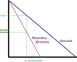
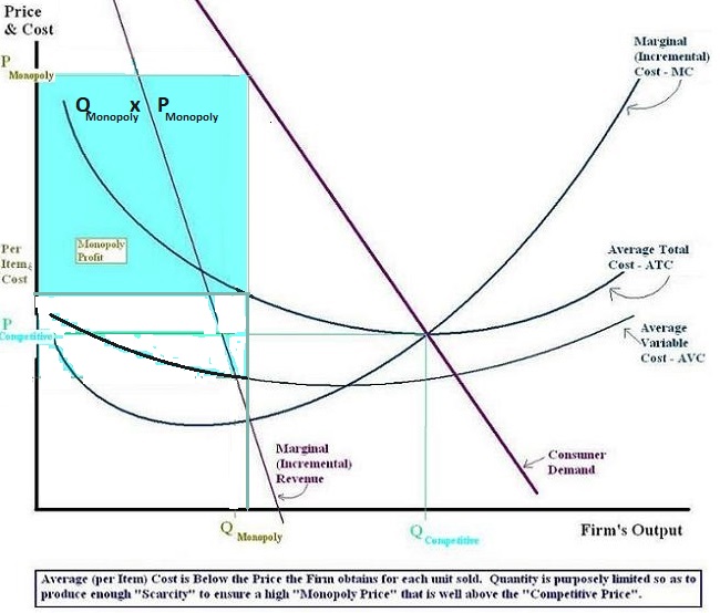
The monopoly ensures a monopoly price exists when it establishes the quantity of the product.[1] As the sole supplier of the product within the market, its sales establish the entire industry's supply within the market, and the monopoly's production and sales decisions can establish a single price for the industry without any influence from competing firms.[1][2][3] The monopoly always considers the demand for its product as it considers what price is appropriate, such that it chooses a production supply and price combination that ensures a maximum economic profit,[1][2] which is determined by ensuring that the marginal cost (determined by the firm's technical limitations that form its cost structure) is the same as the marginal revenue (MR) (as determined by the impact a change in the price of the product will impact the quantity demanded) at the quantity it decides to sell.[1][2] The marginal revenue is solely determined by the demand for the product within the industry and is the change in revenue that will occur by lowering the price just enough to ensure a single additional unit is sold.[1][2] The marginal revenue is positive, but it is lower than its associated price because lowering the price will increase the demand for its product and increase the firm's sales revenue, and lower the price paid by those who are willing to buy the product at the higher price, which ensures a lower sales revenue on the product sales than those willing to pay the higher price.[1]
Marginal revenue can be calculated as [math]\displaystyle{ MR = P + P'(Q) * Q }[/math], where [math]\displaystyle{ 0 \gt P'(Q) }[/math].[2][clarification needed]
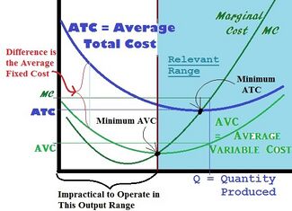
Marginal cost (MC) relates to the firm's technical cost structure within production, and indicates the rise in total cost that must occur for an additional unit to be supplied to the market by the firm.[1] The marginal cost is higher than the average cost because of diminishing marginal product in the short run.[1] It can be calculated as [math]\displaystyle{ MC = C'(Q) }[/math], where [math]\displaystyle{ 0 \lt C'(Q) }[/math].[2][4][clarification needed]

Samuelson[who?] indicates this point on the consumer demand curve is where the price is equal to one over one plus the reciprocal of the price elasticity of demand.[5] This rule does not apply to competitive firms, as they are price takers and do not have the market power to control either prices or industry-wide sales.[1]
Although the term markup is sometimes used in economics to refer to the difference between a monopoly price and the monopoly's MC,[6] it is frequently used in American accounting and finance to define the difference between the price of the product and its per unit accounting cost. Accepted neo-classical micro-economic theory indicates the American accounting and finance definition of markup, as it exists in most competitive markets, ensures an accounting profit that is just enough to solely compensate the equity owners of a competitive firm within a competitive market for the economic cost (opportunity cost) they must bear if they hold on to the firm's equity.[3] The economic cost of holding onto equity at its present value is the opportunity cost the investor must bear when giving up the interest earnings on debt of similar present value (they hold onto equity instead of the debt).[3] Economists would indicate that a markup rule on economic cost used by a monopoly to set a monopoly price that will maximize its profit is excessive markup that leads to inefficiencies within an economic system.[1][2][7][8]
Mathematical derivation: how a monopoly sets the monopoly price
Mathematically, the general rule a monopoly uses to maximize monopoly profit can be derived through simple calculus. The basic equation for economic profit, in which the total economic cost varies directly with the quantity produced, can be expressed as
[math]\displaystyle{ \pi = P(Q)\times Q - C(Q) }[/math], where
- [math]\displaystyle{ Q }[/math] = quantity sold,
- [math]\displaystyle{ P(Q) }[/math] = inverse demand function; the price at which [math]\displaystyle{ Q }[/math] can be sold given the existing demand
- [math]\displaystyle{ C(Q) }[/math] = total cost of producing [math]\displaystyle{ Q }[/math].
- [math]\displaystyle{ \pi }[/math] = economic profit
This is done by equating the derivative of [math]\displaystyle{ \pi }[/math] with respect to [math]\displaystyle{ Q }[/math] to 0. The profit of a firm is given by total revenue (price times quantity sold) minus total cost:
[math]\displaystyle{ P'(Q)Q+P-C'(Q)=0 }[/math], where
- [math]\displaystyle{ Q }[/math] = quantity sold,
- [math]\displaystyle{ P'(Q) }[/math] = the partial derivative of the inverse demand function, and the price at which [math]\displaystyle{ Q }[/math] can be sold given the existing demand
- [math]\displaystyle{ C'(Q) }[/math] = marginal cost, or the partial derivative of the total cost of producing [math]\displaystyle{ Q }[/math]
which yields
[math]\displaystyle{ P'(Q)*Q + P = C'(Q) }[/math]
where marginal revenue equals marginal cost. This is usually called the first order conditions for a profit maximum.[2]
According to Samuelson,
[math]\displaystyle{ P(P'(Q/P)+1)=MC }[/math]
By definition, [math]\displaystyle{ P'(Q/P) }[/math] is the reciprocal of the price elasticity of demand (or [math]\displaystyle{ 1/ \epsilon }[/math]), or
[math]\displaystyle{ P(1+1/{\epsilon})=MC }[/math]
This gives the markup rule:
[math]\displaystyle{ P=\frac {\epsilon} {\epsilon+1} MC }[/math].
Note that the price elasticity of demand (and its reciprocal) is negative, [math]\displaystyle{ {\epsilon}\lt 0 }[/math], so a more intuitive formula, using the absolute value of the elasticity, is
[math]\displaystyle{ P=\frac {|\epsilon|} {|\epsilon|-1} MC }[/math].
This shows clearly that the profit-maximizing price is set at a point where "demand is elastic", namely, the price elasticity of demand must be greater than unity in absolute terms, in order for the profit-maximizing price to be positive.
Letting [math]\displaystyle{ \eta }[/math] be the reciprocal of the price elasticity of demand,
[math]\displaystyle{ P=\frac {1} {1+\eta} MC }[/math]
Thus the monopolistic firm chooses the quantity at which the demand price satisfies this rule. Since [math]\displaystyle{ \eta\lt 0 }[/math] for a price setting firm, it means that a firm with market power will charge a price above marginal cost and earn a monopoly rent. On the other hand, a competitive firm by definition faces a perfectly elastic demand, [math]\displaystyle{ \eta=0 }[/math], which means that it sets price equal to marginal cost.
The rule also implies that, absent menu costs, a monopolistic firm will never choose a point on the inelastic portion of its demand curve. For an equilibrium to exist in a monopoly or in an oligopoly market, the price elasticity of demand must be less than negative one ([math]\displaystyle{ \frac{1}{\eta}\lt -1 }[/math]), for marginal revenue to be positive.[4] The mathematical profit maximization conditions ("first order conditions") ensure the price elasticity of demand must be less than negative one,[2][7] since no rational firm that attempts to maximize its profit would incur additional cost (a positive marginal cost) in order to reduce revenue (when MR < 0).[1]
In the case of price elasticity of demand, it also called Lerner index. The formula can be expressed: [math]\displaystyle{ L = \frac{P - MC}{P} }[/math], [math]\displaystyle{ P }[/math] means monopoly price set by firms [math]\displaystyle{ MC }[/math] means the marginal cost of production
The Lerner index measures the level of market power and monopoly power that a firm owned.The higher Lerner index indicated the more monopoly power allows a company have chance to establish prices that are higher than their marginal costs and then lead a higher monopoly price. In conclusion, a monopoly price is established by a monopolistic firm while they have no rivals in the market and feasible to raise price further above their marginal cost. In order to ensure a maximum economic return, the monopoly price is established at the point where marginal revenue equals marginal cost based on the firm's evaluation of the demand for its product. The Lerner index can be used to measured the degree of monopoly power and monopoly price.
In addition, monopoly price will prevent new business from entering the market and restrict innovation. A monopoly would not like to invest more on research and development or innovation due to it already has a captive market. Then the lack of innovation may block market competition and limit the industry’s growth potential in long run. The monopoly’s entrance restrictions also make it difficult for new businesses to enter the market, which reduces the scope for innovation and new ideas.
In sum up, monopoly pricing generally has negative consequences on consumers and the overall economy, resulting in higher costs, lower quantity desired, inefficiencies and a lack of innovation.
Properties
Objectives
Of the many price-setting methods, a monopoly will set the price with respect to market demand id est demand-based pricing.
When a firm with absolute market power sets the monopoly price, the primary objective is to maximize its own profits by capturing consumer surplus and maximizing its own. A monopoly accomplishes this by setting a price above its marginal cost and producing at a quantity that meets market demand and corresponds to the set price.
Nature
Monopoly Price and market inefficiencies
Monopoly pricing without perfect price discrimination results in market inefficiencies when compared to other market structures. The inefficiencies in question are a loss of both consumer and producer surplus otherwise known as a deadweight loss. The loss in both surplus' are deemed allocatively inefficient and not socially optimal. In contrast, when the firm has more information and discrimination is present, monopoly pricing becomes increasingly efficient as it approaches perfect discrimination through the various forms of price discrimination:
Theoretical Considerations
Dynamic Pricing for Monopolies
Much of the empirical literature suggest that setting a dynamic or variable monopoly price is market-efficient and can maximize total profits for the firm. However, this is only true when certain assumptions are made and specific circumstances are present. A paper written by Harris and Raviv [9] advise firms who are restricted by productive capacity to set their prices on a priority-basis. If production capacity is capped and not only restricted, Harris and Raviv suggest pricing goods in an auction format to be optimal for maximizing profits. Both pricing schemes are argued to be effective under the assumptions that price adjustments are costless. Further studies by Rajan et al. (1993)[10] have also concluded that a variable pricing scheme to be optimal for maximizing profits. Rajan argues that dynamic costs such as purchasing and carrying costs should lead to an increase in price. Additionally, He suggests goods that drop in value or decay should lead to a decrease in price as demand for said goods also decrease therefore the firm should drop the price as to maximize profits again and reclaim lost producer surplus.
Market structure of monopoly
A market structure is defined by three factors which are barriers to entry, number of firms in the market, and product substitutability.
Below is the market structure for a monopoly:
| Barriers to entry[11] | Number of firms in the market | Product substitutability |
|---|---|---|
|
1 | No other perfect substitutes of product |
Unlike perfect competition where firms can freely enter and exit the market, it is not the case for monopolistic competition. For a monopoly to exist, there must be high barriers to entry for new firms. Barriers to entry must be strong enough to discourage potential competitors from entering. However, if the number of firms in the market for a specific good or service increases, the perceived value of firms in the market will decrease. Therefore, the likelihood for firms to exit the market is higher, leaving one firm to monopolise the market.
The difference between the products or services of a perfect competition and one in a monopoly is if the products or services are differentiated. Thereby, the products or services sold in the monopolistic market are not perfect substitutes for one another.[12]
Market power of monopoly
Market power is the firm's ability to affect terms and conditions of exchange. [13] A monopoly possesses a substantial amount of market power, however, it is not unlimited. A monopoly is a price maker, not a price taker, meaning that a monopoly has the power to set the market price. [14] The firm in monopoly is the market as it sets its price based on their circumstances of what best suits them.
Summary of monopoly characteristics
To easily identify a monopoly, it would have one or more of these five characteristics
| Characteristics | Explanation |
|---|---|
| Profit maximiser | Monopolist will maximise their profits by ensuring marginal cost (MC) = marginal revenue (MR). |
| Price Maker | The monopolist sets the price according to its own circumstances and not what other firms are pricing their products or services as. |
| High barriers to entry | Other firms are unable to enter the market of the monopoly |
| Single seller/ firm | The monopolist is the only seller in the market that produces all the outputs meeting all the demands of the market. |
| Price discrimination | The firm in monopoly can change the price and quantity of the product as they please. Therefore, to meet all demands and gain a profit, they may sell high quantities at a low price in an elastic market and sell lower quantities at a high price in an inelastic market. |
References
- ↑ 1.00 1.01 1.02 1.03 1.04 1.05 1.06 1.07 1.08 1.09 1.10 1.11 1.12 1.13 Roger LeRoy Miller, Intermediate Microeconomics Theory Issues Applications, Third Edition, New York: McGraw-Hill, Inc, 1982.
- ↑ 2.00 2.01 2.02 2.03 2.04 2.05 2.06 2.07 2.08 2.09 2.10 2.11 Tirole, Jean, "The Theory of Industrial Organization", Cambridge, Massachusetts: The MIT Press, 1988.
- ↑ 3.0 3.1 3.2 John Black, "Oxford Dictionary of Economics", New York: Oxford University Press, 2003.
- ↑ 4.0 4.1 Henderson, James M., and Richard E. Quandt, "Micro Economic Theory, A Mathematical Approach. 3rd Edition", New York: McGraw-Hill Book Company, 1980. Glenview, Illinois: Scott, Foresmand and Company, 1988.
Usually, in many textbooks, economic cost, here presented by [math]\displaystyle{ C(Q) }[/math], is divided into two categories; labor costs and capital costs:
[math]\displaystyle{ C(Q) = Lw + K R }[/math], where
- [math]\displaystyle{ L }[/math] = labor hired,
- [math]\displaystyle{ w }[/math] = wage rate,
- [math]\displaystyle{ K }[/math] = total amount of capital financed by both debt and equity,
- [math]\displaystyle{ R }[/math] = cost of capital, including both interest expense and the minimum required rate of return on equity
- [math]\displaystyle{ Q }[/math] = [math]\displaystyle{ Q(L,K) }[/math] = a function of the quantity of labor and capital employed in production
- ↑ Samuelson; Marks (2003). p.104
- ↑ Nicholson, Walter and Christopher Snyder, Microeconomic Theory: Basic Principles and Extensions, Mason, OH: Thomson/South-Western, 2008.
- ↑ 7.0 7.1 Henderson, James M., and Richard E. Quandt, "Micro Economic Theory, A Mathematical Approach. 3rd Edition", New York: McGraw-Hill Book Company, 1980. Glenview, Illinois: Scott, Foresmand and Company, 1988.
- ↑ Bradley R. chiller, "Essentials of Economics", New York: McGraw-Hill, Inc., 1991.
- ↑ Harris, Milton; Raviv, Artur (1981). "A Theory of Monopoly Pricing Schemes with Demand Uncertainty". The American Economic Review 71 (3): 347–365. ISSN 0002-8282. https://www.jstor.org/stable/1802784.
- ↑ Rajan, Arvind; Steinberg, Rakesh; Steinberg, Richard (1992). "Dynamic Pricing and Ordering Decisions by a Monopolist". Management Science 38 (2): 240–262. ISSN 0025-1909. https://www.jstor.org/stable/2632506.
- ↑ Samuelson, William F; Marks, Stephen G (2003). Managerial Economics. Wiley. pp. 365–366. ISBN 978-0-470-00041-0.
- ↑ Hirschey (2000). Managerial Economics. Dreyden. p. 426.
- ↑ Krugman, Paul; Wells, Robin (2009). Microeconomics (2nd ed.). Worth.
- ↑ Melvin, Michael; Boyes, William (2002). Microeconomics (5th ed.). Houghton Mifflin. p. 239.
 |


