Generalized chi-squared distribution

Generalized chi-squared distribution

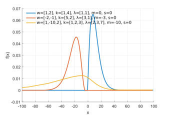
Probability density function
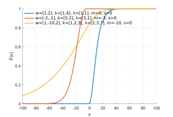
Cumulative distribution function
Notation	[math]\displaystyle{ \tilde{\chi}(\boldsymbol{w}, \boldsymbol{k}, \boldsymbol{\lambda},s,m) }[/math]
Parameters	[math]\displaystyle{ \boldsymbol{w} }[/math], vector of weights of noncentral chi-square components [math]\displaystyle{ \boldsymbol{k} }[/math], vector of degrees of freedom of noncentral chi-square components [math]\displaystyle{ \boldsymbol{\lambda} }[/math], vector of non-centrality parameters of chi-square components [math]\displaystyle{ s }[/math], scale of normal term [math]\displaystyle{ m }[/math], offset
Support	[math]\displaystyle{ x \in \begin{cases} [m, +\infty) \text{ if } w_i \geq 0, s=0,\\ (-\infty,m] \text{ if } w_i \leq 0, s=0,\\ \R \text{ otherwise.} \end{cases} }[/math]
Mean	[math]\displaystyle{ \sum_j w_j (k_j+\lambda_j)+m }[/math]
Variance	[math]\displaystyle{ 2 \sum_j w_j^2 (k_j+2 \lambda_j) + s^2 }[/math]
CF	[math]\displaystyle{ \frac{\exp\left[it \left( m + \sum_j \frac{w_j \lambda_j}{1-2i w_j t} \right)-\frac{s^2 t^2}{2}\right]}{\prod_j \left(1-2i w_j t \right)^{k_j/2}} }[/math]

In probability theory and statistics, the generalized chi-squared distribution (or generalized chi-square distribution) is the distribution of a quadratic form of a multinormal variable (normal vector), or a linear combination of different normal variables and squares of normal variables. Equivalently, it is also a linear sum of independent noncentral chi-square variables and a normal variable. There are several other such generalizations for which the same term is sometimes used; some of them are special cases of the family discussed here, for example the gamma distribution.

Definition

The generalized chi-squared variable may be described in multiple ways. One is to write it as a weighted sum of independent noncentral chi-square variables [math]\displaystyle{ {{\chi}'}^2 }[/math] and a standard normal variable [math]\displaystyle{ z }[/math]:

[math]\displaystyle{ \tilde{\chi}(\boldsymbol{w}, \boldsymbol{k}, \boldsymbol{\lambda},s,m)=\sum_i w_i {{\chi}'}^2 (k_i,\lambda_i) + sz+m. }[/math]

Here the parameters are the weights [math]\displaystyle{ w_i }[/math], the degrees of freedom [math]\displaystyle{ k_i }[/math] and non-centralities [math]\displaystyle{ \lambda_i }[/math] of the constituent non-central chi-squares, and the coefficients [math]\displaystyle{ s }[/math] and [math]\displaystyle{ m }[/math] of the normal. Some important special cases of this have all weights [math]\displaystyle{ w_i }[/math] of the same sign, or have central chi-squared components, or omit the normal term.

Since a non-central chi-squared variable is a sum of squares of normal variables with different means, the generalized chi-square variable is also defined as a sum of squares of independent normal variables, plus an independent normal variable: that is, a quadratic in normal variables.

Another equivalent way is to formulate it as a quadratic form of a normal vector [math]\displaystyle{ \boldsymbol{x} }[/math]:

[math]\displaystyle{ \tilde{\chi}=q(\boldsymbol{x}) = \boldsymbol{x}' \mathbf{Q_2} \boldsymbol{x} + \boldsymbol{q_1}' \boldsymbol{x} + q_0 }[/math].

Here [math]\displaystyle{ \mathbf{Q_2} }[/math] is a matrix, [math]\displaystyle{ \boldsymbol{q_1} }[/math] is a vector, and [math]\displaystyle{ q_0 }[/math] is a scalar. These, together with the mean [math]\displaystyle{ \boldsymbol{\mu} }[/math] and covariance matrix [math]\displaystyle{ \mathbf{\Sigma} }[/math] of the normal vector [math]\displaystyle{ \boldsymbol{x} }[/math], parameterize the distribution. The parameters of the former expression (in terms of non-central chi-squares, a normal and a constant) can be calculated in terms of the parameters of the latter expression (quadratic form of a normal vector). If (and only if) [math]\displaystyle{ \mathbf{Q_2} }[/math] in this formulation is positive-definite, then all the [math]\displaystyle{ w_i }[/math] in the first formulation will have the same sign.

For the most general case, a reduction towards a common standard form can be made by using a representation of the following form:

[math]\displaystyle{ X=(z+a)^\mathrm T A(z+a)+c^\mathrm T z= (x+b)^\mathrm T D(x+b)+d^\mathrm T x+e , }[/math]

where D is a diagonal matrix and where x represents a vector of uncorrelated standard normal random variables.

Computing the pdf/cdf/inverse cdf/random numbers

The probability density, cumulative distribution, and inverse cumulative distribution functions of a generalized chi-squared variable do not have simple closed-form expressions. However, numerical algorithms and computer code (Fortran and C, Matlab, R, Python) have been published to evaluate some of these, and to generate random samples.

In the case where [math]\displaystyle{ \boldsymbol{q_1} = 0 }[/math], it is possible to obtain an exact expression for the mean and variance of [math]\displaystyle{ \xi }[/math], as shown in the article on quadratic forms.

Applications

The generalized chi-squared is the distribution of statistical estimates in cases where the usual statistical theory does not hold, as in the examples below.

In model fitting and selection

If a predictive model is fitted by least squares, but the residuals have either autocorrelation or heteroscedasticity, then alternative models can be compared (in model selection) by relating changes in the sum of squares to an asymptotically valid generalized chi-squared distribution.

Classifying normal vectors using Gaussian discriminant analysis

If [math]\displaystyle{ \boldsymbol{x} }[/math] is a normal vector, its log likelihood is a quadratic form of [math]\displaystyle{ \boldsymbol{x} }[/math], and is hence distributed as a generalized chi-squared. The log likelihood ratio that [math]\displaystyle{ \boldsymbol{x} }[/math] arises from one normal distribution versus another is also a quadratic form, so distributed as a generalized chi-squared.

In Gaussian discriminant analysis, samples from multinormal distributions are optimally separated by using a quadratic classifier, a boundary that is a quadratic function (e.g. the curve defined by setting the likelihood ratio between two Gaussians to 1). The classification error rates of different types (false positives and false negatives) are integrals of the normal distributions within the quadratic regions defined by this classifier. Since this is mathematically equivalent to integrating a quadratic form of a normal vector, the result is an integral of a generalized-chi-squared variable.

In signal processing

The following application arises in the context of Fourier analysis in signal processing, renewal theory in probability theory, and multi-antenna systems in wireless communication. The common factor of these areas is that the sum of exponentially distributed variables is of importance (or identically, the sum of squared magnitudes of circularly-symmetric centered complex Gaussian variables).

If [math]\displaystyle{ Z_i }[/math] are k independent, circularly-symmetric centered complex Gaussian random variables with mean 0 and variance [math]\displaystyle{ \sigma_i^2 }[/math], then the random variable

[math]\displaystyle{ \tilde{Q} = \sum_{i=1}^k |Z_i|^2 }[/math]

has a generalized chi-squared distribution of a particular form. The difference from the standard chi-squared distribution is that [math]\displaystyle{ Z_i }[/math] are complex and can have different variances, and the difference from the more general generalized chi-squared distribution is that the relevant scaling matrix A is diagonal. If [math]\displaystyle{ \mu=\sigma_i^2 }[/math] for all i, then [math]\displaystyle{ \tilde{Q} }[/math], scaled down by [math]\displaystyle{ \mu/2 }[/math] (i.e. multiplied by [math]\displaystyle{ 2/\mu }[/math]), has a chi-squared distribution, [math]\displaystyle{ \chi^2(2k) }[/math], also known as an Erlang distribution. If [math]\displaystyle{ \sigma_i^2 }[/math] have distinct values for all i, then [math]\displaystyle{ \tilde{Q} }[/math] has the pdf

[math]\displaystyle{ f(x; k,\sigma_1^2,\ldots,\sigma_k^2) = \sum_{i=1}^k \frac{e^{-\frac x {\sigma_i^2}}}{\sigma_i^2 \prod_{j=1, j\neq i}^k \left(1- \frac{\sigma_j^2}{\sigma_i^2}\right)} \quad\text{for } x\geq0. }[/math]

If there are sets of repeated variances among [math]\displaystyle{ \sigma_i^2 }[/math], assume that they are divided into M sets, each representing a certain variance value. Denote [math]\displaystyle{ \mathbf{r}=(r_1, r_2, \dots, r_M) }[/math] to be the number of repetitions in each group. That is, the mth set contains [math]\displaystyle{ r_m }[/math] variables that have variance [math]\displaystyle{ \sigma^2_m. }[/math] It represents an arbitrary linear combination of independent [math]\displaystyle{ \chi^2 }[/math]-distributed random variables with different degrees of freedom:

[math]\displaystyle{ \tilde{Q} = \sum_{m=1}^M \sigma^2_m/2* Q_m, \quad Q_m \sim \chi^2(2r_m) \, . }[/math]

The pdf of [math]\displaystyle{ \tilde{Q} }[/math] is

[math]\displaystyle{ f(x; \mathbf{r}, \sigma^2_1, \dots \sigma^2_M) = \prod_{m=1}^M \frac{1}{\sigma^{2r_m}_m} \sum_{k=1}^M \sum_{l=1}^{r_k} \frac{\Psi_{k,l,\mathbf{r}}}{(r_k-l)!} (-x)^{r_k-l} e^{-\frac{x}{\sigma^2_k}}, \quad \text{ for }x\geq0 , }[/math]

where

[math]\displaystyle{ \Psi_{k,l,\mathbf{r}} = (-1)^{r_k-1} \sum_{\mathbf{i} \in \Omega_{k,l}} \prod_{j \neq k} \binom{i_j + r_j-1}{i_j} \left(\frac 1 {\sigma^2_j}\!-\!\frac{1}{\sigma^2_k} \right)^{-(r_j + i_j)}, }[/math]

with [math]\displaystyle{ \mathbf{i}=[i_1,\ldots,i_M]^T }[/math] from the set [math]\displaystyle{ \Omega_{k,l} }[/math] of all partitions of [math]\displaystyle{ l-1 }[/math] (with [math]\displaystyle{ i_k=0 }[/math]) defined as

[math]\displaystyle{ \Omega_{k,l} = \left\{ [i_1,\ldots,i_m]\in \mathbb{Z}^m; \sum_{j=1}^M i_j \!= l-1, i_k=0, i_j\geq 0 \text{ for all } j \right\}. }[/math]

See also

• Degrees of freedom (statistics)
• Noncentral chi-squared distribution
• Chi-squared distribution

External links

• Davies, R.B.: Fortran and C source code for "Linear combination of chi-squared random variables"
• Das, A: MATLAB code to compute the statistics, pdf, cdf, inverse cdf and random numbers of the generalized chi-square distribution.

References

- ↑ Davies, R.B. (1973) Numerical inversion of a characteristic function. Biometrika, 60 (2), 415–417
- ↑ 2.0 2.1 Davies, R.B. (1980) "Algorithm AS155: The distribution of a linear combination of χ2 random variables", Applied Statistics, 29, 323–333
- ↑ 3.0 3.1 Jones, D.A. (1983) "Statistical analysis of empirical models fitted by optimisation", Biometrika, 70 (1), 67–88
- ↑ 4.0 4.1 4.2 4.3 4.4 Das, Abhranil; Wilson S Geisler (2020). "Methods to integrate multinormals and compute classification measures". arXiv:2012.14331 [stat.ML].
- ↑ 5.0 5.1 Sheil, J., O'Muircheartaigh, I. (1977) "Algorithm AS106: The distribution of non-negative quadratic forms in normal variables",Applied Statistics, 26, 92–98
- ↑ Imhof, J. P. (1961). "Computing the Distribution of Quadratic Forms in Normal Variables". Biometrika 48 (3/4): 419–426. doi:10.2307/2332763. http://doc.rero.ch/record/294852/files/48-3-4-419.pdf.
- ↑ D. Hammarwall, M. Bengtsson, B. Ottersten (2008) "Acquiring Partial CSI for Spatially Selective Transmission by Instantaneous Channel Norm Feedback", IEEE Transactions on Signal Processing, 56, 1188–1204
- ↑ E. Björnson, D. Hammarwall, B. Ottersten (2009) "Exploiting Quantized Channel Norm Feedback through Conditional Statistics in Arbitrarily Correlated MIMO Systems", IEEE Transactions on Signal Processing, 57, 4027–4041