Lyapunov fractal
In mathematics, Lyapunov fractals (also known as Markus–Lyapunov fractals) are bifurcational fractals derived from an extension of the logistic map in which the degree of the growth of the population, r, periodically switches between two values A and B.[1]
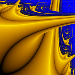
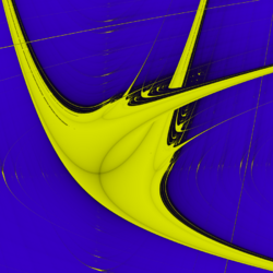
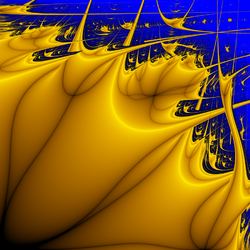
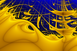
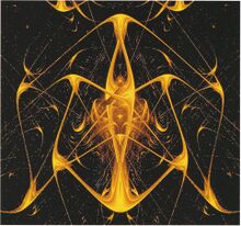
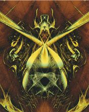
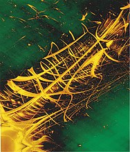
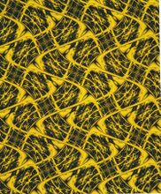
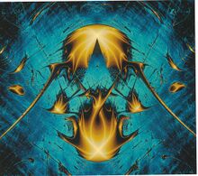
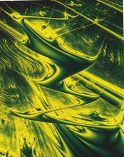
A Lyapunov fractal is constructed by mapping the regions of stability and chaotic behaviour (measured using the Lyapunov exponent [math]\displaystyle{ \lambda }[/math]) in the a−b plane for given periodic sequences of a and b. In the images, yellow corresponds to [math]\displaystyle{ \lambda \lt 0 }[/math] (stability), and blue corresponds to [math]\displaystyle{ \lambda \gt 0 }[/math] (chaos).
Lyapunov fractals were discovered in the late 1980s[2] by the Germano-Chilean physicist Mario Markus from the Max Planck Institute of Molecular Physiology. They were introduced to a large public by a science popularization article on recreational mathematics published in Scientific American in 1991.[3]
Properties
Lyapunov fractals are generally drawn for values of A and B in the interval [math]\displaystyle{ [0,4] }[/math]. For larger values, the interval [0,1] is no longer stable, and the sequence is likely to be attracted by infinity, although convergent cycles of finite values continue to exist for some parameters. For all iteration sequences, the diagonal a = b is always the same as for the standard one parameter logistic function.
The sequence is usually started at the value 0.5, which is a critical point of the iterative function.[4] The other (even complex valued) critical points of the iterative function during one entire round are those that pass through the value 0.5 in the first round. A convergent cycle must attract at least one critical point.[5] Therefore, all convergent cycles can be obtained by just shifting the iteration sequence, and keeping the starting value 0.5. In practice, shifting this sequence leads to changes in the fractal, as some branches get covered by others. For instance, the Lyapunov fractal for the iteration sequence AB (see top figure on the right) is not perfectly symmetric with respect to a and b.
Algorithm
The algorithm for computing Lyapunov fractals works as follows:[6]
- Choose a string of As and Bs of any nontrivial length (e.g., AABAB).
- Construct the sequence [math]\displaystyle{ S }[/math] formed by successive terms in the string, repeated as many times as necessary.
- Choose a point [math]\displaystyle{ (a,b) \in [0,4] \times [0,4] }[/math].
- Define the function [math]\displaystyle{ r_n = a }[/math] if [math]\displaystyle{ S_n = A }[/math], and [math]\displaystyle{ r_n = b }[/math] if [math]\displaystyle{ S_n = B }[/math].
- Let [math]\displaystyle{ x_0 = 0.5 }[/math], and compute the iterates [math]\displaystyle{ x_{n+1} = r_n x_n (1 - x_n) }[/math].
- Compute the Lyapunov exponent:
[math]\displaystyle{ \lambda = \lim_{N \rightarrow \infty} {1 \over N} \sum_{n = 1}^N \log \left|{dx_{n+1} \over dx_n}\right| = \lim_{N \rightarrow \infty} {1 \over N} \sum_{n = 1}^N \log |r_n (1 - 2x_n)| }[/math]
In practice, [math]\displaystyle{ \lambda }[/math] is approximated by choosing a suitably large [math]\displaystyle{ N }[/math] and dropping the first summand as [math]\displaystyle{ r_0 (1 - 2x_0) = r_n \cdot 0 = 0 }[/math] for [math]\displaystyle{ x_0=0.5 }[/math]. - Color the point [math]\displaystyle{ (a,b) }[/math] according to the value of [math]\displaystyle{ \lambda }[/math] obtained.
- Repeat steps (3–7) for each point in the image plane.
More Iterations
More dimensions
File:Lyapunov fractal animation.webm Lyapunov fractals can be calculated in more than two dimensions. The sequence string for a n-dimensional fractal has to be built from an alphabet with n characters, e.g. "ABBBCA" for a 3D fractal, which can be visualized either as 3D object or as an animation showing a "slice" in the C direction for each animation frame, like the example given here.
Notes
- ↑ See Markus & Hess 1989, p. 553.
- ↑ See Markus & Hess 1989 and Markus 1990.
- ↑ See Dewdney 1991.
- ↑ See Markus 1990, p. 483.
- ↑ See Markus 1990, p. 486.
- ↑ See Markus 1990, pp. 481,483 and Markus & Hess 1998.
References
- Dewdney, A.K. (1991). "Leaping into Lyapunov Space". Scientific American 265 (3): 130–132. doi:10.1038/scientificamerican0991-178.
- Markus, Mario; Hess, Benno (1989). "Lyapunov exponents of the logistic map with periodic forcing". Computers and Graphics 13 (4): 553–558. doi:10.1016/0097-8493(89)90019-8.
- Markus, Mario (1990). "Chaos in Maps with Continuous and Discontinuous Maxima". Computers in Physics 4 (5): 481. doi:10.1063/1.4822940.
- Markus, Mario; Hess, Benno (1998). "Chapter 12. Lyapunov exponents of the logistic map with periodic forcing". in Clifford A. Pickover. Chaos and Fractals. A Computer Graphical Journey. Elsevier. pp. 73-78. doi:10.1016/B978-0-444-50002-1.X5000-0. ISBN 978-0-444-50002-1. https://archive.org/details/chaosfractalscom00pick.
- Markus, Mario, "Die Kunst der Mathematik", Verlag Zweitausendeins, Frankfurt ISBN:978-3-86150-767-3
External links
- EFG's Fractals and Chaos – Lyapunov Exponents
- Elert, Glenn. "Lyapunov Space". The Chaos Hypertextbook. http://hypertextbook.com/chaos/lyapunov-2/.
 |
