ProbOnto

Short description: Knowledge base and ontology of probability distributions

ProbOnto
Keywords	Statistics, Probability distribution
Objective	Design, implement and maintain knowledge base and ontology of probability distributions.
Duration	2015 –
Website	probonto.org

ProbOnto is a knowledge base and ontology of probability distributions. ProbOnto 2.5 (released on January 16, 2017) contains over 150 uni- and multivariate distributions and alternative parameterizations, more than 220 relationships and re-parameterization formulas, supporting also the encoding of empirical and univariate mixture distributions.

Introduction

ProbOnto was initially designed to facilitate the encoding of nonlinear-mixed effect models and their annotation in Pharmacometrics Markup Language (PharmML) developed by DDMoRe, an Innovative Medicines Initiative project. However, ProbOnto, due to its generic structure can be applied in other platforms and modeling tools for encoding and annotation of diverse models applicable to discrete (e.g. count, categorical and time-to-event) and continuous data.

Knowledge base

Overview of supported distributions in ProbOnto, version 2.5, and relationships between univariate probability distributions.

The knowledge base stores for each distribution:

• Probability density or mass functions and where available cumulative distribution, hazard and survival functions.
• Related quantities such as mean, median, mode and variance.
• Parameter and support/range definitions and distribution type.
• LaTeX and R code for mathematical functions.
• Model definition and references.

Relationships

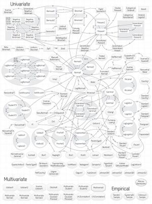
ProbOnto stores in Version 2.5 over 220 relationships between univariate distributions with re-parameterizations as a special case, see figure. While this form of relationships is often neglected in literature, and the authors concentrate one a particular form for each distribution, they are crucial from the interoperability point of view. ProbOnto focuses on this aspect and features more than 15 distributions with alternative parameterizations.

Alternative parameterizations

Many distributions are defined with mathematically equivalent but algebraically different formulas. This leads to issues when exchanging models between software tools. The following examples illustrate that.

Normal distribution

Normal distribution can be defined in at least three ways

• Normal1(μ,σ) with mean, μ, and standard deviation, σ

[math]\displaystyle{ P(x;\boldsymbol\mu,\boldsymbol\sigma)= \frac{1}{\sigma \sqrt{2 \pi}}\exp\Big[-\frac{(x-\mu)^2}{2\sigma^2}\Big] }[/math]

• Normal2(μ,υ) with mean, μ, and variance, υ = σ^2 or

[math]\displaystyle{ P(x;\boldsymbol\mu,\boldsymbol v)= \frac{1}{\sqrt{v} \sqrt{2 \pi}}\exp\Big[-\frac{(x-\mu)^2}{2v}\Big] }[/math]

• Normal3(μ,τ) with mean, μ, and precision, τ = 1/υ = 1/σ^2.

[math]\displaystyle{ P(x;\boldsymbol\mu,\boldsymbol\tau)= \sqrt{\frac{\tau}{2 \pi}} \Big[-\frac{\tau}{2}(x-\mu)^2\Big] }[/math]

Re-parameterization formulas

The following formulas can be used to re-calculate the three different forms of the normal distribution (we use abbreviations i.e. [math]\displaystyle{ N1 }[/math] instead of [math]\displaystyle{ Normal1 }[/math] etc.)

• [math]\displaystyle{ N1(\mu,\sigma) \rightarrow N2(\mu,v): v=\sigma^2 \mbox{ and } N2(\mu,v) \rightarrow N1(\mu,\sigma): \sigma=\sqrt{v}; }[/math]

• [math]\displaystyle{ N1(\mu,\sigma) \rightarrow N3(\mu,\tau): \tau=1/\sigma^2 \mbox{ and } N3(\mu,\tau) \rightarrow N1(\mu,\sigma): \sigma=1/\sqrt{\tau}; }[/math]

• [math]\displaystyle{ N2(\mu,v) \rightarrow N3(\mu,\tau): \tau=1/v \mbox{ and } N3(\mu,\tau) \rightarrow N2(\mu,v): v=1/\tau. }[/math]

Log-normal distribution

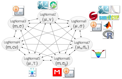
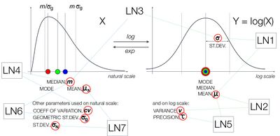
In the case of the log-normal distribution there are more options. This is due to the fact that it can be parameterized in terms of parameters on the natural and log scale, see figure.

Overview of parameterizations of the log-normal distributions.

Support of different parameterizations of the log-normal distributions in various tools and there connections, see text for examples. Tools visualised are Matlab (supports LN1), MCSim (LN6), Monolix (LN2 & LN3), PFIM (LN2 & LN3), Phoenix NLME (LN1, LN3 & LN6), PopED (LN7), R (programming language) (LN1), Simcyp Simulator (LN1), Simulx (LN1) and winBUGS (LN5)

The available forms in ProbOnto 2.0 are

• LogNormal1(μ,σ) with mean, μ, and standard deviation, σ, both on the log-scale

[math]\displaystyle{ P(x;\boldsymbol\mu,\boldsymbol\sigma)= \frac{1}{x \sigma \sqrt{2 \pi}} \exp\Big[ \frac{-(\log x - \mu)^2}{2\sigma^2}\Big] }[/math]

• LogNormal2(μ,υ) with mean, μ, and variance, υ, both on the log-scale

[math]\displaystyle{ P(x;\boldsymbol\mu,\boldsymbol {v})=\frac{1}{x \sqrt{v} \sqrt{2 \pi}} \exp\Big[ \frac{-(\log x - \mu)^2}{2 v}\Big] }[/math]

• LogNormal3(m,σ) with median, m, on the natural scale and standard deviation, σ, on the log-scale

[math]\displaystyle{ P(x;\boldsymbol m,\boldsymbol \sigma) =\frac{1}{x \sigma \sqrt{2 \pi}} \exp\Big[ \frac{-[\log(x/m)]^2}{2\sigma^2}\Big] }[/math]

• LogNormal4(m,cv) with median, m, and coefficient of variation, cv, both on the natural scale

[math]\displaystyle{ P(x;\boldsymbol m,\boldsymbol {cv})= \frac{1}{x \sqrt{\log(cv^2+1)} \sqrt{2 \pi}} \exp\Big[ \frac{-[\log(x/m)]^2}{2\log(cv^2+1)}\Big] }[/math]

• LogNormal5(μ,τ) with mean, μ, and precision, τ, both on the log-scale

[math]\displaystyle{ P(x;\boldsymbol\mu,\boldsymbol \tau)=\sqrt{\frac{\tau}{2 \pi}} \frac{1}{x} \exp\Big[ {-\frac{\tau}{2}(\log x-\mu)^2} \Big] }[/math]

• LogNormal6(m,σ_g) with median, m, and geometric standard deviation, σ_g, both on the natural scale

[math]\displaystyle{ P(x;\boldsymbol m,\boldsymbol {\sigma_g})=\frac{1}{x \log(\sigma_g)\sqrt{2 \pi}} \exp\Big[ \frac{-[\log(x/m)]^2}{2 \log^2(\sigma_g)}\Big] }[/math]

• LogNormal7(μ_N,σ_N) with mean, μ_N, and standard deviation, σ_N, both on the natural scale

[math]\displaystyle{ P(x;\boldsymbol {\mu_N},\boldsymbol {\sigma_N})= \frac{1}{x \sqrt{2 \pi \log\Big(1+\sigma_N^2/\mu_N^2\Big)}} \exp\Bigg( \frac{-\Big[ \log(x) - \log\Big(\frac{\mu_N}{\sqrt{1+\sigma_N^2/\mu_N^2}}\Big)\Big]^2}{2\log\Big(1+\sigma_N^2/\mu_N^2\Big)}\Bigg) }[/math]

ProbOnto knowledge base stores such re-parameterization formulas to allow for a correct translation of models between tools.

Examples for re-parameterization

Consider the situation when one would like to run a model using two different optimal design tools, e.g. PFIM and PopED. The former supports the LN2, the latter LN7 parameterization, respectively. Therefore, the re-parameterization is required, otherwise the two tools would produce different results.

For the transition [math]\displaystyle{ LN2(\mu, v) \rightarrow LN7(\mu_N, \sigma_N) }[/math] following formulas hold [math]\displaystyle{ \mu_N = \exp(\mu+v/2) \text{ and } \sigma_N = \exp(\mu+v/2)\sqrt{\exp(v)-1} }[/math].

For the transition [math]\displaystyle{ LN7(\mu_N, \sigma_N) \rightarrow LN2(\mu, v) }[/math] following formulas hold [math]\displaystyle{ \mu = \log\Big( \mu_N/\sqrt{1+\sigma_N^2/\mu_N^2} \Big) \text{ and } v = \log(1+\sigma_N^2/\mu_N^2) }[/math].

All remaining re-parameterisation formulas can be found in the specification document on the project website.

Ontology

The knowledge base is built from a simple ontological model. At its core, a probability distribution is an instance of the class thereof, a specialization of the class of mathematical objects. A distribution relates to a number of other individuals, which are instances of various categories in the ontology. For example, these are parameters and related functions associated with a given probability distribution. This strategy allows for the rich representation of attributes and relationships between domain objects. The ontology can be seen as a conceptual schema in the domain of mathematics and has been implemented as a PowerLoom knowledge base. An OWL version is generated programmatically using the Jena API.

Output for ProbOnto are provided as supplementary materials and published on or linked from the probonto.org website. The OWL version of ProbOnto is available via Ontology Lookup Service (OLS) to facilitate simple searching and visualization of the content. In addition the OLS API provides methods to programmatically access ProbOnto and to integrate it into applications. ProbOnto is also registered on the BioSharing portal.

ProbOnto in PharmML

A PharmML interface is provided in form of a generic XML schema for the definition of the distributions and their parameters. Defining functions, such as probability density function (PDF), probability mass function (PMF), hazard function (HF) and survival function (SF), can be accessed via methods provided in the PharmML schema.

Use example

This example shows how the zero-inflated Poisson distribution is encoded by using its codename and declaring that of its parameters (‘rate’ and ‘probabilityOfZero’). Model parameters Lambda and P0 are assigned to the parameter code names.

<Distribution>
    <po:ProbOnto name="ZeroInflatedPoisson1">
        <po:Parameter name="rate">
            <ct:Assign>
                <ct:SymbRef symbIdRef="Lambda" />
            </ct:Assign>
        </po:Parameter>
        <po:Parameter name="probabilityOfZero">
            <ct:Assign>
                <ct:SymbRef symbIdRef="P0" />
            </ct:Assign>
        </po:Parameter>
    </po:ProbOnto>
</Distribution>

To specify any given distribution unambiguously using ProbOnto, it is sufficient to declare its code name and the code names of its parameters. More examples and a detailed specification can be found on the project website.

See also

• List of probability distributions
• Ontology (computer science)
• Relationships among probability distributions
• Web Ontology Language

External links

• ProbOnto website
• Leemis chart
• Ultimate Univariate Probability Distribution Explorer – most likely the largest, free collection of univariate distributions and their features.
• UncertML

References

- ↑ Swat, MJ; Grenon, P; Wimalaratne, S (2016). "ProbOnto: ontology and knowledge base of probability distributions". Bioinformatics 32: 2719. doi:10.1093/bioinformatics/btw170. PMID 27153608.
- ↑ 2.0 2.1 2.2 Main project website, URL: http://probonto.org
- ↑ Swat MJ. et al. (2015). Pharmacometrics Markup Language (PharmML): Opening New Perspectives for Model Exchange in Drug Development. CPT Pharmacometrics Syst Pharmacol, 4(6):316-9.
- ↑ PharmML website, URL: http://pharmml.org
- ↑ DDMoRe project website, URL: http://ddmore.eu
- ↑ ProbOnto description on the DDMoRe website, URL: http://ddmore.eu/probonto
- ↑ LeBauer DS et al. Translating probability density functions: From R to BUGS and back again, R Journal, 2013
- ↑ 8.0 8.1 8.2 Forbes et al. Probability Distributions (2011), John Wiley & Sons, Inc.
- ↑ Wolfram Mathworld, URL: http://mathworld.wolfram.com/NormalDistribution.html
- ↑ 'LaplacesDemon' R package, URL: http://search.r-project.org/library/LaplacesDemon/html/dist.Normal.Precision.html
- ↑ Cyert RM, MH DeGroot, Bayesian Analysis and Uncertainty in Economic (1987), TheoryRowman & Littlefield
- ↑ Lunn, D. (2012). The BUGS book: a practical introduction to Bayesian analysis. Texts in statistical science. CRC Press.
- ↑ Limpert, E., Stahel, W. A., and Abbt, M. (2001). Log-normal distributions across the sciences: Keys and clues. BioScience, 51(5):341-352.
- ↑ Nyberg J. et al. (2012) PopED - An extended, parallelized, population optimal design tool. Comput Methods Programs Biomed.; 108(2):789-805. doi: 10.1016/j.cmpb.2012.05.005
- ↑ Retout S, Duffull S, Mentré F (2001) Development and implementation of the population Fisher information matrix for the evaluation of population pharmacokinetic designs. Comp Meth Pro Biomed 65:141–151
- ↑ The PopED Development Team (2016). PopED Manual, Release version 2.13. Technical report, Uppsala University.
- ↑ MacGregor R. et al. (1997) Powerloom Manual. ISI, University of South California, Marina del Rey.
- ↑ McBride B. (2001) Jena: Implementing the RDF model and syntax specification. In: SemWeb.
- ↑ ProbOnto on Ontology Lookup Service, URL: http://www.ebi.ac.uk/ols/ontologies/probonto
- ↑ ProbOnto on BioSharing, the database of biological databases, URL: https://biosharing.org/biodbcore-000772