Mixed model

Short description: Statistical model containing both fixed effects and random effects

A mixed model, mixed-effects model or mixed error-component model is a statistical model containing both fixed effects and random effects. These models are useful in a wide variety of disciplines in the physical, biological and social sciences. They are particularly useful in settings where repeated measurements are made on the same statistical units (longitudinal study), or where measurements are made on clusters of related statistical units. Mixed models are often preferred over traditional analysis of variance regression models because of their flexibility in dealing with missing values and uneven spacing of repeated measurements. The Mixed model analysis allows measurements to be explicitly modeled in a wider variety of correlation and variance-covariance structures.

This page will discuss mainly linear mixed-effects models (LMEM) rather than generalized linear mixed models or nonlinear mixed-effects models.

Qualitative Description

Linear mixed models (LMMs) are statistical models that incorporate fixed and random effects to accurately represent non-independent data structures. LMM is an alternative to analysis of variance. Often, ANOVA assumes the independence of observations within each group, however, this assumption may not hold in non-independent data, such as multilevel/hierarchical, longitudinal, or correlated datasets.

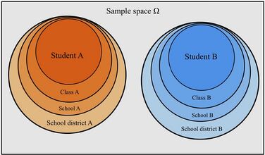
Non-independent sets are ones in which the variability between outcomes is due to correlations within groups or between groups. Mixed models properly account for nest structures/hierarchical data structures where observations are influenced by their nested associations. For example, when studying education methods involving multiple schools, there are multiple levels of variables to consider. The individual level/lower level comprises individual students or teachers within the school. The observations obtained from this student/teacher is nested within their school. For example, Student A is a unit within the School A. The next higher level is the school. At the higher level, the school contains multiple individual students and teachers. The school level influences the observations obtained from the students and teachers. For Example, School A and School B are the higher levels each with its set of Student A and Student B respectively. This represents a hierarchical data scheme. A solution to modeling hierarchical data is using linear mixed models.

Representation of how data, related to education system, is non-independent and structured in nested/hierarchial levels.

LMMs allow us to understand the important effects between and within levels while incorporating the corrections for standard errors for non-independence embedded in the data structure.

The Fixed Effect

Fixed effects encapsulate the tendencies/trends that are consistent at the levels of primary interest. These effects are considered fixed because they are non-random and assumed to be constant for the population being studied. For example, when studying education a fixed effect could represent overall school level effects that are consistent across all schools.

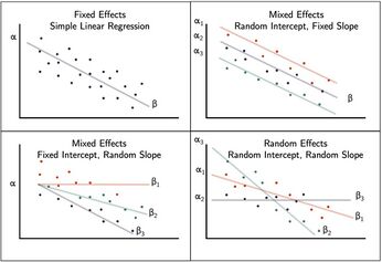
While the hierarchy of the data set is typically obvious, the specific fixed effects that affect the average responses for all subjects must be specified. Some fixed effect coefficients are sufficient without corresponding random effects where as other fixed coefficients only represent an average where the individual units are random. These may be determined by incorporating random intercepts and slopes.

In most situations, several related models are considered and the model that best represents a universal model is adopted.

The Random Effect, ε

A key component of the mixed model is the incorporation of random effects with the fixed effect. Fixed effects are often fitted to represent the underlying model. In Linear mixed models, the true regression of the population is linear, β. The fixed data is fitted at the highest level. Random effects introduce statistical variability at different levels of the data hierarchy. These account for the unmeasured sources of variance that affect certain groups in the data. For example, the differences between student 1 and student 2 in the same class, or the differences between class 1 and class 2 in the same school.  

History and current status

Representation of biased vs. unbiased data and the differences between LSR and LMM fitted estimates.

Ronald Fisher introduced random effects models to study the correlations of trait values between relatives. In the 1950s, Charles Roy Henderson provided best linear unbiased estimates of fixed effects and best linear unbiased predictions of random effects. Subsequently, mixed modeling has become a major area of statistical research, including work on computation of maximum likelihood estimates, non-linear mixed effects models, missing data in mixed effects models, and Bayesian estimation of mixed effects models. Mixed models are applied in many disciplines where multiple correlated measurements are made on each unit of interest. They are prominently used in research involving human and animal subjects in fields ranging from genetics to marketing, and have also been used in baseball and industrial statistics. The mixed linear model association has improved the prevention of false positive associations. Populations are deeply interconnected and the relatedness structure of population dynamics is extremely difficult to model without the use of mixed models. Linear mixed models may not, however, be the only solution. LMM's have a constant-residual variance assumption that is sometimes violated when accounting or deeply associated continuous and binary traits.

Definition

In matrix notation a linear mixed model can be represented as

[math]\displaystyle{ \boldsymbol{y} = X \boldsymbol{\beta} + Z \boldsymbol{u} + \boldsymbol{\epsilon} }[/math]

where

• [math]\displaystyle{ \boldsymbol{y} }[/math] is a known vector of observations, with mean [math]\displaystyle{ E(\boldsymbol{y}) = X \boldsymbol{\beta} }[/math];
• [math]\displaystyle{ \boldsymbol{\beta} }[/math] is an unknown vector of fixed effects;
• [math]\displaystyle{ \boldsymbol{u} }[/math] is an unknown vector of random effects, with mean [math]\displaystyle{ E(\boldsymbol{u})=\boldsymbol{0} }[/math] and variance–covariance matrix [math]\displaystyle{ \operatorname{var}(\boldsymbol{u})=G }[/math];
• [math]\displaystyle{ \boldsymbol{\epsilon} }[/math] is an unknown vector of random errors, with mean [math]\displaystyle{ E(\boldsymbol{\epsilon})=\boldsymbol{0} }[/math] and variance [math]\displaystyle{ \operatorname{var}(\boldsymbol{\epsilon})=R }[/math];
• [math]\displaystyle{ X }[/math] is the known design matrix for the fixed effects relating the observations [math]\displaystyle{ \boldsymbol{y} }[/math] to [math]\displaystyle{ \boldsymbol{\beta} }[/math], respectively
• [math]\displaystyle{ Z }[/math] is the known design matrix for the random effects relating the observations [math]\displaystyle{ \boldsymbol{y} }[/math] to [math]\displaystyle{ \boldsymbol{u} }[/math], respectively.

Estimation

The joint density of [math]\displaystyle{ \boldsymbol{y} }[/math] and [math]\displaystyle{ \boldsymbol{u} }[/math] can be written as: [math]\displaystyle{ f(\boldsymbol{y},\boldsymbol{u}) = f(\boldsymbol{y} | \boldsymbol{u}) \, f(\boldsymbol{u}) }[/math]. Assuming normality, [math]\displaystyle{ \boldsymbol{u} \sim \mathcal{N}(\boldsymbol{0},G) }[/math], [math]\displaystyle{ \boldsymbol{\epsilon} \sim \mathcal{N}(\boldsymbol{0},R) }[/math] and [math]\displaystyle{ \mathrm{Cov}(\boldsymbol{u},\boldsymbol{\epsilon})=\boldsymbol{0} }[/math], and maximizing the joint density over [math]\displaystyle{ \boldsymbol{\beta} }[/math] and [math]\displaystyle{ \boldsymbol{u} }[/math], gives Henderson's "mixed model equations" (MME) for linear mixed models:

[math]\displaystyle{ \begin{pmatrix} X'R^{-1}X & X'R^{-1}Z \\ Z'R^{-1}X & Z'R^{-1}Z + G^{-1} \end{pmatrix} \begin{pmatrix} \hat{\boldsymbol{\beta}} \\ \hat{\boldsymbol{u}} \end{pmatrix} = \begin{pmatrix} X'R^{-1}\boldsymbol{y} \\ Z'R^{-1}\boldsymbol{y} \end{pmatrix} }[/math]

The solutions to the MME, [math]\displaystyle{ \textstyle\hat{\boldsymbol{\beta}} }[/math] and [math]\displaystyle{ \textstyle\hat{\boldsymbol{u}} }[/math] are best linear unbiased estimates and predictors for [math]\displaystyle{ \boldsymbol{\beta} }[/math] and [math]\displaystyle{ \boldsymbol{u} }[/math], respectively. This is a consequence of the Gauss–Markov theorem when the conditional variance of the outcome is not scalable to the identity matrix. When the conditional variance is known, then the inverse variance weighted least squares estimate is best linear unbiased estimates. However, the conditional variance is rarely, if ever, known. So it is desirable to jointly estimate the variance and weighted parameter estimates when solving MMEs.

One method used to fit such mixed models is that of the expectation–maximization algorithm (EM) where the variance components are treated as unobserved nuisance parameters in the joint likelihood. Currently, this is the method implemented in statistical software such as Python (statsmodels package) and SAS (proc mixed), and as initial step only in R's nlme package lme(). The solution to the mixed model equations is a maximum likelihood estimate when the distribution of the errors is normal.

Fixed, mixed, and random effects influence linear regression models.

There are several other methods to fit mixed models, including using an MEM initially, and then Newton-Raphson (used by R package nlme's lme()), penalized least squares to get a profiled log likelihood only depending on the (low-dimensional) variance-covariance parameters of [math]\displaystyle{ \boldsymbol{u} }[/math], i.e., its cov matrix [math]\displaystyle{ \boldsymbol{G} }[/math], and then modern direct optimization for that reduced objective function (used by R's lme4 package lmer() and the Julia package MixedModels.jl) and direct optimization of the likelihood (used by e.g. R's glmmTMB). Notably, while the canonical form proposed by Henderson is useful for theory, many popular software packages use a different formulation for numerical computation in order to take advantage of sparse matrix methods (e.g. lme4 and MixedModels.jl).

See also

• Nonlinear mixed-effects model
• Fixed effects model
• Generalized linear mixed model
• Linear regression
• Mixed-design analysis of variance
• Multilevel model
• Random effects model
• Repeated measures design
• Empirical Bayes method

Further reading

• Gałecki, Andrzej; Burzykowski, Tomasz (2013). Linear Mixed-Effects Models Using R: A Step-by-Step Approach. New York: Springer. ISBN 978-1-4614-3900-4. 
• Milliken, G. A.; Johnson, D. E. (1992). Analysis of Messy Data: Vol. I. Designed Experiments. New York: Chapman & Hall. 
• West, B. T.; Welch, K. B.; Galecki, A. T. (2007). Linear Mixed Models: A Practical Guide Using Statistical Software. New York: Chapman & Hall/CRC.

References

- ↑ Baltagi, Badi H. (2008). Econometric Analysis of Panel Data (Fourth ed.). New York: Wiley. pp. 54–55. ISBN 978-0-470-51886-1.
- ↑ 2.0 2.1 Gomes, Dylan G.E. (20 January 2022). "Should I use fixed effects or random effects when I have fewer than five levels of a grouping factor in a mixed-effects model?". PeerJ 10. doi:10.7717/peerj.12794. PMID 35116198.
- ↑ Yang, Jian; Zaitlen, NA; Goddard, ME; Visscher, PM; Prince, AL (29 January 2014). "Advantages and pitfalls in the application of mixed-model association methods". Nat Genet 46 (2): 100–106. doi:10.1038/ng.2876. PMID 24473328.
- ↑ 4.0 4.1 Seltman, Howard (2016). Experimental Design and Analysis. 1. pp. 357–378. https://www.stat.cmu.edu/~hseltman/309/Book/.
- ↑ 5.0 5.1 "Introduction to Linear Mixed Models". Advanced Research Computing Statistical Methods and Data Analytics. UCLA Statistical Consulting Group. 2021. https://stats.oarc.ucla.edu/other/mult-pkg/introduction-to-linear-mixed-models/.
- ↑ Judd, Charles M.; Westfall, Jacob; Kenny, David A. (2012). "Treating stimuli as a random factor in social psychology: A new and comprehensive solution to a pervasive but largely ignored problem.". Journal of Personality and Social Psychology 103 (1): 54–69. doi:10.1037/a0028347. PMID 22612667.
- ↑ Boisgontier, Matthieu P.; Cheval, Boris (September 2016). "The anova to mixed model transition" (in en). Neuroscience & Biobehavioral Reviews 68: 1004–1005. doi:10.1016/j.neubiorev.2016.05.034. PMID 27241200. https://linkinghub.elsevier.com/retrieve/pii/S0149763416301634.
- ↑ Schmidt-Catran, Alexander W.; Fairbrother, Malcolm (February 2016). "The Random Effects in Multilevel Models: Getting Them Wrong and Getting Them Right". European Sociological Review 32 (1): 23–38. doi:10.1093/esr/jcv090.
- ↑ 9.0 9.1 Kreft & de Leeuw, J.. Introducing multilevel modeling. London:Sage.
- ↑ 10.0 10.1 Raudenbush, Bryk, S.W, A.S (2002). Hierarchical Linear Models: Applications and Data Analysis Methods. Thousand Oaks, CA: Sage.
- ↑ 11.0 11.1 Snijders, Bosker, T.A.B, R.J (2012). Multilevel analysis: An introduction to basic and advanced multilevel modeling. 2nd edition. London:Sage.
- ↑ Fisher, RA (1918). "The correlation between relatives on the supposition of Mendelian inheritance". Transactions of the Royal Society of Edinburgh 52 (2): 399–433. doi:10.1017/S0080456800012163. https://zenodo.org/record/1428666.
- ↑ 13.0 13.1 Robinson, G.K. (1991). "That BLUP is a Good Thing: The Estimation of Random Effects". Statistical Science 6 (1): 15–32. doi:10.1214/ss/1177011926.
- ↑ C. R. Henderson; Oscar Kempthorne; S. R. Searle; C. M. von Krosigk (1959). "The Estimation of Environmental and Genetic Trends from Records Subject to Culling". Biometrics (International Biometric Society) 15 (2): 192–218. doi:10.2307/2527669.
- ↑ 15.0 15.1 L. Dale Van Vleck. "Charles Roy Henderson, April 1, 1911 – March 14, 1989". United States National Academy of Sciences. https://www.nasonline.org/wp-content/uploads/2024/06/henderson-charles.pdf.
- ↑ McLean, Robert A.; Sanders, William L.; Stroup, Walter W. (1991). "A Unified Approach to Mixed Linear Models". The American Statistician (American Statistical Association) 45 (1): 54–64. doi:10.2307/2685241.
- ↑ Anderson, R.J (2016). ""MLB analytics guru who could be the next Nate Silver has a revolutionary new stat"". http://www.cbssports.com/mlb/news/mlb-analytics-guru-who-could-be-the-next-nate-silver-has-a-revolutionary-new-stat/.
- ↑ Obenchain, Bob; Lilly, Eli (1993). "Data Analysis and Information Visualization". MWSUG. https://www.lexjansen.com/mwsug/1993/MWSUG93035.pdf.
- ↑ Chen, H; Wang, C; Conomos, MP; Stilp, AM; Li, Z; Sofer, T; Szpiro, AA; Chen, W et al. (7 April 2016). "Control for Population Structure and Relatedness for Binary Traits in Genetic Association Studies via Logistic Mixed Models". Am J Hum Genet 98 (4): 653–666. doi:10.1016/j.ajhg.2016.02.012. PMID 27018471.
- ↑ Henderson, C R (1973). "Sire evaluation and genetic trends". Journal of Animal Science (American Society of Animal Science) 1973: 10–41. doi:10.1093/ansci/1973.Symposium.10. http://www.journalofanimalscience.org/content/1973/Symposium/10.full.pdf. Retrieved 17 August 2014.
- ↑ Barr, Dale J.; Levy, Roger; Scheepers, Christoph; Tily, Harry J. (April 2013). "Random effects structure for confirmatory hypothesis testing: Keep it maximal". Journal of Memory and Language 68 (3): 255–278. doi:10.1016/j.jml.2012.11.001. PMID 24403724.
- ↑ Lindstrom, ML; Bates, DM (1988). "Newton–Raphson and EM algorithms for linear mixed-effects models for repeated-measures data". Journal of the American Statistical Association 83 (404): 1014–1021. doi:10.1080/01621459.1988.10478693.
- ↑ Laird, Nan M.; Ware, James H. (1982). "Random-Effects Models for Longitudinal Data". Biometrics (International Biometric Society) 38 (4): 963–974. doi:10.2307/2529876. PMID 7168798.
- ↑ Fitzmaurice, Garrett M.; Laird, Nan M.; Ware, James H. (2004). Applied Longitudinal Analysis. John Wiley & Sons. pp. 326–328.
- ↑ Pinheiro, J; Bates, DM (2006). Mixed-effects models in S and S-PLUS. Statistics and Computing. New York: Springer Science & Business Media. doi:10.1007/b98882. ISBN 0-387-98957-9.
- ↑ Bates, D.; Maechler, M.; Bolker, B.; Walker, S. (2015). "Fitting Linear Mixed-Effects Models Using lme4". Journal of Statistical Software 67 (1). doi:10.18637/jss.v067.i01.
- ↑ Bürkner, Paul-Christian (2017). "brms : An R Package for Bayesian Multilevel Models Using Stan". Journal of Statistical Software 80 (1). doi:10.18637/jss.v080.i01.
- ↑ Bürkner, Paul-Christian (2018). "Advanced Bayesian Multilevel Modeling with the R Package brms". The R Journal 10 (1): 395. doi:10.32614/RJ-2018-017.
- ↑ Capretto, Tomás; Piho, Camen; Kumar, Ravin; Westfall, Jacob; Yarkoni, Tal; Martin, Osvaldo A. (2020). "Bambi: A simple interface for fitting Bayesian linear models in Python". arXiv:2012.10754 [stat.CO].