Hardy distribution

Short description: Discrete probability distribution

Hardy Distribution

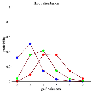
Probability mass function The horizontal axis represents the hole score n. The vertical axis represents the probability of the hole score n given the par of the hole and the probabilities p = 0.20 and q = 0.10. The blue points represent the probabilities for a par three, the green points for a par four and the red points for a par five The function is defined only at integer values of n. The connecting lines are only guides for the eye.
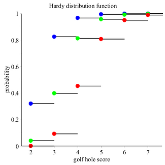
Cumulative distribution function The horizontal axis represents the hole score n. The vertical axis represents the cumulative probability of the hole score n given the par of the hole and the probabilities p = 0.20 and q = 0.10. The blue points represent the probabilities for a par three, the green points for a par four and the red points for a par five. The cumulative probability density (CDF) is discontinuous at the integers of n and flat everywhere else because a variable that is Hardy distributed takes on only integer values.
Notation	[math]\displaystyle{ \operatorname{Hardy}(p, q; m) }[/math]
Parameters	[math]\displaystyle{ p, q\in (0, 1) }[/math], [math]\displaystyle{ p + q\in (0, 1) }[/math] and [math]\displaystyle{ m = 1, 2, 3, \dots }[/math]
Support	[math]\displaystyle{ n \in \mathbb{N}_0 }[/math] (Natural numbers starting from 1)
pmf	For m is odd: [math]\displaystyle{ P \left( X=n \right) \, = \,\sum _{j=\frac{m+1}{2}}^{m}{n-1\choose n-j}{q}^{n-j} \left( A_{{j,m}}+B_{{j,m}} \right) }[/math] For m is even: [math]\displaystyle{ P \left( X=n \right) \, = \,\sum _{j=\frac{m}{2}}^{m}{n-1\choose n-j}{q}^{n-j} \left( A_{{j,m}}+B_{{j,m}} \right) }[/math] with [math]\displaystyle{ A_{{j,m}}\, = \, {j-1\choose 2\,j-m-1}{p}^{m-j+1} \left( 1-p-q \right) ^{2\,j-m-1} }[/math] and [math]\displaystyle{ B_{{j,m}}\, = \, {j\choose 2\,j-m}{p}^{m-j} \left( 1-p-q \right) ^{2\,j-m} }[/math]
Mean	[math]\displaystyle{ \, - \, \sum _{j=1}^{m}{\frac { \left( m+1-j \right) \, {p}^{j-1}}{ \left( q-1 \right) ^{j}}} }[/math]
MGF	For m is odd: [math]\displaystyle{ M _{m }\left(t \right)=\sum _{j=\frac{m}{2}+\frac{1}{2}}^{m}\frac{\left(X _{{\it jm} }+Y _{{\it jm} }\right)~e^{j ~t }}{\left(1-e^{t }~q \right)^{j }} }[/math] For m is even: [math]\displaystyle{ M _{m }\left(t \right)=\sum _{j=\frac{m}{2}}^{m}\frac{\left(X _{{\it jm} }+Y _{{\it jm} }\right)~e^{j ~t }}{\left(1-e^{t }~q \right)^{j }} }[/math] with [math]\displaystyle{ X_{{{\it jm}}}\, = \,{j-1\choose 2\,j-m-1}{p}^{m+1-j} \left( 1-p-q \right) ^{2\,j-m-1} }[/math] and [math]\displaystyle{ Y_{{{\it jm}}}\, = \,{j\choose 2\,j-m}{p}^{-j+m} \left( 1-p-q \right) ^{2\,j-m} }[/math]

In probability theory and statistics, the Hardy distribution is a discrete probability distribution that expresses the probability of the hole score for a given golf player. It is based on Hardy's (Hardy, 1945) basic assumption that there are three types of shots:

good [math]\displaystyle{ (G) }[/math], 
bad [math]\displaystyle{ (B) }[/math] and 
ordinary [math]\displaystyle{ (O) }[/math], 

where the probability of a good hit equals [math]\displaystyle{ p }[/math], the probability of a bad hit equals [math]\displaystyle{ q }[/math] and the probability of an ordinary hit equals [math]\displaystyle{ 1 - p - q }[/math]. Hardy further assigned

a value of 2 to a good stroke, 
a value of 0 to a bad stroke and 
a value of 1 to a regular or ordinary stroke. 

Once the sum of the values is greater than or equal to the value of the par of the hole, the number of strokes in question is equal to the score achieved on that hole. A birdie on a par three could then have come about in three ways: [math]\displaystyle{ OG }[/math], [math]\displaystyle{ GO }[/math] and [math]\displaystyle{ GG }[/math], respectively, with probabilities [math]\displaystyle{ (1-p-q) \, p }[/math], [math]\displaystyle{ p \, (1-p-q) }[/math] and [math]\displaystyle{ p^2 }[/math].

Definitions

Probability mass function

A discrete random variable X is said to have a Hardy distribution, with parameters [math]\displaystyle{ p }[/math], [math]\displaystyle{ q }[/math] and [math]\displaystyle{ m }[/math] if it has a probability mass function given by:

[math]\displaystyle{ P \left( X=n \right) \, = \,\sum _{j=\frac{m+1}{2}}^{m}{n-1\choose n-j}{q}^{n-j} \left( A_{{j,m}}+B_{{j,m}} \right) }[/math] if m is odd

and

[math]\displaystyle{ P \left( X=n \right) \, = \,\sum _{j=\frac{m}{2}}^{m}{n-1\choose n-j}{q}^{n-j} \left( A_{{j,m}}+B_{{j,m}} \right) }[/math] if m is even

with

[math]\displaystyle{ A_{{j,m}}\, = \, {j-1\choose 2\,j-m-1}{p}^{m-j+1} \left( 1-p-q \right) ^{2\,j-m-1} }[/math]

and

[math]\displaystyle{ B_{{j,m}}\, = \, {j\choose 2\,j-m}{p}^{m-j} \left( 1-p-q \right) ^{2\,j-m} }[/math]

where

• m is the par of the hole ([math]\displaystyle{ m = 1, 2, \ldots }[/math])

• n is the golf hole score ([math]\displaystyle{ n = \frac{m}{2}, \frac{m}{2} + 1, \frac{m}{2} + 2, \ldots }[/math]) if [math]\displaystyle{ m }[/math] is even

• n is the golf hole score ([math]\displaystyle{ n = \frac{m+1}{2}, \frac{m+1}{2} + 1, \frac{m+1}{2} + 2, \ldots }[/math]) if [math]\displaystyle{ m }[/math] is odd

• p is the probability of a good shot ([math]\displaystyle{ 0 \lt p \lt 1 }[/math])

• q is the probability of a bad shot ([math]\displaystyle{ 0 \lt q \lt 1 }[/math]) and ([math]\displaystyle{ 0 \lt p+q \lt 1 }[/math])

The moment generating function is given by:

[math]\displaystyle{ M _{m }\left(t \right)=\sum _{j=\frac{m}{2}+\frac{1}{2}}^{m}\frac{\left(X _{{\it jm} }+Y _{{\it jm} }\right)~e^{j ~t }}{\left(1-e^{t }~q \right)^{j }} }[/math] if m is odd

and

[math]\displaystyle{ M _{m }\left(t \right)=\sum _{j=\frac{m}{2}}^{m}\frac{\left(X _{{\it jm} }+Y _{{\it jm} }\right)~e^{j ~t }}{\left(1-e^{t }~q \right)^{j }} }[/math] if m is even

with

[math]\displaystyle{ X_{{{\it jm}}}\, = \,{j-1\choose 2\,j-m-1}{p}^{m+1-j} \left( 1-p-q \right) ^{2\,j-m-1} }[/math]

and

[math]\displaystyle{ Y_{{{\it jm}}}\, = \,{j\choose 2\,j-m}{p}^{-j+m} \left( 1-p-q \right) ^{2\,j-m} }[/math]

Each raw moment and each central moment can be easily determined with the moment generating function, but the formulas involved are too large to present here.

Hardy distribution for a par three, four and five

For a par three:

[math]\displaystyle{ \begin{align} P \left( T_{{3}}=n \right) &= {n-1\choose n-2} {q}^{n-2} \left( {p}^{2}+2\,p \, \left( 1-p-q \right) \right)+\\ &+{n-1\choose n-3}{q}^{n-3} \left( p \, \left( 1-p-q \right) ^{2}+ \left( 1-p-q \right) ^{3} \right) \end{align} }[/math]

For a par four:

[math]\displaystyle{ \begin{align} P \left( T_{{4}}=n \right) &= {n-1\choose n-2} {q}^{n-2}{p}^{2}+\\ &+{n-1\choose n-3}{q}^{n-3} \left( 2\,{p}^{2} \left( 1-p-q \right) +3\,p \, \left( 1-p-q \right) ^{2} \right)+\\ &+{n-1\choose n-4}{q}^{n-4} \left( p \, \left( 1-p-q \right) ^{3}+ \left( 1-p-q \right) ^{4} \right) \end{align} }[/math]

Note the resemblance with [math]\displaystyle{ P(T_{3}=n) }[/math]. For a par five:

[math]\displaystyle{ \begin{align} P \left( T_{{5}}=n \right) &= {n-1\choose n-3}{q}^{n-3} \left( {p}^{3}+3\,{p}^{2} \left( 1-p-q \right) \right) +\\ &+{n-1\choose n-4}{q}^{n-4} \left( 3\,{p}^{2} \left( 1-p-q \right) ^{2}+4\,p \, \left( 1-p-q \right) ^{3} \right) +\\ &+{n-1\choose n-5}{q}^{n-5} \left( p \, \left( 1-p-q \right) ^{4}+ \left( 1-p-q \right) ^{5} \right) \end{align} }[/math]

Note the resemblance with the formulas for [math]\displaystyle{ P(T_{3}=n) }[/math] and [math]\displaystyle{ P(T_{4}=n) }[/math].

History

When trying to make a probability distribution in golf that describes the frequency distribution of the number of strokes on a hole, the simplest setup is to assume that there are only two types of strokes:

A good stroke with a probability of [math]\displaystyle{ p }[/math]  
A bad stroke with a probability of [math]\displaystyle{ 1-p }[/math]. 
while
a good shot then gets the value 1 and
a bad shot gets the value 0. 

Once the sum of the shot values equals the par of the hole, that is the number of strokes needed for the hole. It is clear that with this setup, a birdie is not possible. After all, the smallest number of strokes one can get is the par of the hole. Hardy (1945) probably realized that too and then came up with the idea not to assume that there were just two types of strokes: good [math]\displaystyle{ (G) }[/math] and bad [math]\displaystyle{ (B) }[/math], but three types:

good [math]\displaystyle{ (G) }[/math] with probability [math]\displaystyle{ p }[/math]    
bad [math]\displaystyle{ (B) }[/math] with probability [math]\displaystyle{ q }[/math]    
ordinary [math]\displaystyle{ (O) }[/math] with probability [math]\displaystyle{ 1-p-q }[/math].   

In fact, Hardy called a good shot a supershot and a bad shot a subshot. Minton later called Hardy's supershot an excellent shot [math]\displaystyle{ (E) }[/math] and Hardy's subshot a bad shot [math]\displaystyle{ (B) }[/math]. In this article, Minton's excellent shot is called a good shot [math]\displaystyle{ (G) }[/math]. Hardy came up with the idea of three types of shots in 1945, but the actual derivation of the probability distribution of the hole score was not given until 2012 by van der Ven.

Hardy assumed that the probability of a good stroke was equal to the probability of a bad stroke, namely [math]\displaystyle{ p = q }[/math]. This was confirmed by Kang:

Hardy's model is very simple in that all strokes are independent from each other and the probability of producing a good shot is equal to the probability of producing a bad shot.

In retrospect, Hardy might well have been right, as the data in Table 2 in van der Ven (2013) show. This table shows the estimated [math]\displaystyle{ p }[/math]- and [math]\displaystyle{ q }[/math]-values for holes 1-18 for rounds 1 and 2 of the 2012 British Open Championship. The mean values were equal to 0.0633 and 0.0697, respectively. Later Cohen (2002) introduced the idea that [math]\displaystyle{ p }[/math] and [math]\displaystyle{ q }[/math] should be different. Kang says about this:

Cohen takes another step forward and includes the possibility that the probability of good shots and bad shots can differ.

For the Hardy distribution the values of [math]\displaystyle{ p }[/math] and [math]\displaystyle{ q }[/math] may be different.

Goodness of fit

The Hardy distribution gives the probability distribution of a single player's hole score. It takes several observations to perform a goodness-of-fit test (see Goodness of fit test) to check whether the Hardy distribution applies or not. This can be done with a single individual by having the individual play the same hole multiple times. Goodness-of-fit tests assume pure replications (see Replication (statistics)). This means that there should be no change in the player's golfing ability during repeated play of the hole. For example, there should not be an ongoing learning process (see Learning). Such effects cannot really be ruled out. One way around this problem is to use multiple players who can be assumed to have approximately the same golf proficiency. Such players are the participants in professional golf tournaments (see PGA Tour). Before using a goodness-of-fit test, it should first be checked that the participants indeed have approximately the same golf proficiency. This can be done separately for each hole by using, for example, the Pearson correlation coefficient between the hole score on the first day and the second day of a tournament. If there are no systematic differences (see Classical test theory) between players, the correlation (see Correlation) between the score achieved on Day 1 on a hole and the score achieved on Day 2 on that hole will not differ significantly (see Statistical significance) from zero. This can be easily tested statistically. In a study by van der Ven, the results of a goodness-of-fit test of the Hardy distribution were reported using the hole-by-hole scores from the 2012 Open Championship played at the St Andrews Golf Club. The distribution has been tested separately for each hole. Pearson's chi-squared test was used to determine whether the observed sample frequencies of the hole scores differed significantly from the expected frequencies according to the Hardy distribution. The fit between observed and expected frequencies was generally very satisfactory.

References

Notes

References

Notes
- ↑ Hardy, G.H. (1945). "A mathematical theorem about golf". The Mathematical Gazette 29: 226–227. doi:10.2307/3609265.
- ↑ Minton, R. B. (2010). "G. H. Hardy's Golfing Adventure". in Gallian, Joseph A.. Mathematics and sports. Mathematical Association of America. doi:10.5948/UPO9781614442004. ISBN 9780883853498.
- ↑ van der Ven, A.H.G.S. (2012). "The Hardy distribution for golf hole-by-hole scores". The Mathematical Gazette 96: 428–438. doi:10.1017/S0025557200005052.
- ↑ 4.0 4.1 Kang, J. (2017). "Brilliance or steadiness? A suggestion of an alternative model to Hardy's model concerning golf (1945)". The Mathematical Gazette 101 (551): 250–260. doi:10.1017/mag.2017.64.
- ↑ van der Ven, A.H.G.S. (2013). "Applying the Hardy Distribution to the Hole Scores of the 2012 British Open Championship". International Journal of Golf Science 2 (2): 152–161. doi:10.1123/ijgs.2013-0014.