Astronomy:Gauss's method
In orbital mechanics (a subfield of celestial mechanics), Gauss's method is used for preliminary orbit determination from at least three observations (more observations increases the accuracy of the determined orbit) of the orbiting body of interest at three different times. The required information are the times of observations, the position vectors of the observation points (in Equatorial Coordinate System), the direction cosine vector of the orbiting body from the observation points (from Topocentric Equatorial Coordinate System) and general physical data.
Carl Friedrich Gauss developed important mathematical techniques (summed up in Gauss's methods) which were specifically used to determine the orbit of Ceres. The method shown following is the orbit determination of an orbiting body about the focal body where the observations were taken from, whereas the method for determining Ceres' orbit requires a bit more effort because the observations were taken from Earth while Ceres orbits the Sun.
Observer position vector
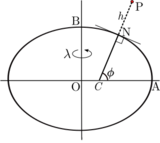
The observer position vector (in Equatorial coordinate system) of the observation points can be determined from the latitude and local sidereal time (from Topocentric coordinate system) at the surface of the focal body of the orbiting body (for example, the Earth) via either:
or where,
- is the respective observer position vector (in Equatorial Coordinate System)
- is the equatorial radius of the central body (e.g., 6,378 km for Earth)
- is the geocentric distance
- is the oblateness (or flattening) of the central body (e.g., 0.003353 for Earth)
- is the eccentricity of the central body (e.g., 0.081819 for Earth)
- is the geodetic latitude (the angle between the normal line of horizontal plane and the equatorial plane)
- is the geocentric latitude (the angle between the radius and the equatorial plane)
- is the geodetic altitude
- is the local sidereal time of observation site
Orbiting body direction cosine vector

The orbiting body direction cosine vector can be determined from the right ascension and declination (from Topocentric Equatorial Coordinate System) of the orbiting body from the observation points via:
where,
- is the respective unit vector in the direction of the position vector (from observation point to orbiting body in Topocentric Equatorial Coordinate System)
- is the respective declination
- is the respective right ascension
Algorithm
The initial derivation begins with vector addition to determine the orbiting body's position vector. Then based on the conservation of angular momentum and Keplerian orbit principles (which states that an orbit lies in a two dimensional plane in three dimensional space), a linear combination of said position vectors is established. Also, the relation between a body's position and velocity vector by Lagrange coefficients is used which results in the use of said coefficients. Then with vector manipulation and algebra, the following equations were derived. For detailed derivation, refer to Curtis.[1]
NOTE: Gauss's method is a preliminary orbit determination, with emphasis on preliminary. The approximation of the Lagrange coefficients and the limitations of the required observation conditions (i.e., insignificant curvature in the arc between observations, refer to Gronchi[2] for more details) causes inaccuracies. Gauss's method can be improved, however, by increasing the accuracy of sub-components, such as solving Kepler's equation. Another way to increase the accuracy is through more observations.
Step 1
Calculate time intervals, subtract the times between observations: where
- is the time interval
- is the respective observation time
Step 2

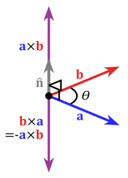
Calculate cross products, take the cross products of the observational unit direction (order matters): where
- is the cross product of vectors
- is the respective cross product vector
- is the respective unit vector
Step 3

Calculate common scalar quantity (scalar triple product), take the dot product of the first observational unit vector with the cross product of the second and third observational unit vector:
where
- is the dot product of vectors and
- is the common scalar triple product
- is the respective cross product vector
- is the respective unit vector
Step 4
Calculate nine scalar quantities (similar to step 3): where
- is the respective scalar quantities
- is the respective observer position vector
- is the respective cross product vector
Step 5
Calculate scalar position coefficients:
where
- , , and are scalar position coefficients
- is the common scalar quantity
- is the respective scalar quantities
- is the time interval
- is the respective observer position vector
- is the respective unit vector
Step 6
Calculate the squared scalar distance of the second observation, by taking the dot product of the position vector of the second observation: where
- is the squared distance of the second observation
- is the position vector of the second observation
Step 7
Calculate the coefficients of the scalar distance polynomial for the second observation of the orbiting body: where
- are coefficients of the scalar distance polynomial for the second observation of the orbiting body
- are scalar position coefficients
- is the gravitational parameter of the focal body of the orbiting body
Step 8
Find the root of the scalar distance polynomial for the second observation of the orbiting body: where
- is the scalar distance for the second observation of the orbiting body (it and its vector, r2, are in the Equatorial Coordinate System)
- are coefficients as previously stated
Various methods can be used to find the root, a suggested method is the Newton–Raphson method. The root must be physically possible (i.e., not negative nor complex) and if multiple roots are suitable, each must be evaluated and compared to any available data to confirm their validity.
Step 9
Calculate the slant range, the distance from the observer point to the orbiting body at their respective time: where
- is the respective slant range (it and its vector, , are in the Topocentric Equatorial Coordinate System)
- is the common scalar quantity
- is the respective scalar quantities
- is the time interval.
- is the scalar distance for the second observation of the orbiting body
- is the gravitational parameter of the focal body of the orbiting body
Step 10
Calculate the orbiting body position vectors, by adding the observer position vector to the slant direction vector (which is the slant distance multiplied by the slant direction vector):
where
- is the respective orbiting body position vector (in Equatorial Coordinate System)
- is the respective observer position vector
- is the respective slant range
- is the respective unit vector
Step 11
Calculate the Lagrange coefficients: where,
- , , and are the Lagrange coefficients (these are just the first two terms of the series expression based on the assumption of small time interval)
- is the gravitational parameter of the focal body of the orbiting body
- is the scalar distance for the second observation of the orbiting body
- is the time interval
Step 12
Calculate the velocity vector for the second observation of the orbiting body:
where
- is the velocity vector for the second observation of the orbiting body (in Equatorial Coordinate System)
- , , and are the Lagrange coefficients
- is the respective orbiting body position vector
Step 13
The orbital state vectors have now been found, the position (r2) and velocity (v2) vector for the second observation of the orbiting body. With these two vectors, the orbital elements can be found and the orbit determined.
See also
References
- ↑ Curtis, Howard D. Orbital Mechanics for Engineering Students. Oxford: Elsevier Butterworth-Heinemann, 2005. Print.
- ↑ Gronchi, Giovanni F.. "Classical and modern orbit determination for asteroids." Proceedings of the International Astronomical Union2004.IAUC196 (2004): 1-11. Print.
- Der, Gim J.. "New Angles-only Algorithms for Initial Orbit Determination." Advanced Maui Optical and Space Surveillance Technologies Conference. (2012). Print.
 |


