Biconnected component

Short description: Maximal biconnected subgraph

Each color corresponds to a biconnected component. Multi-colored vertices are cut vertices, and thus belong to multiple biconnected components.

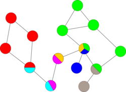
In graph theory, a biconnected component (sometimes known as a 2-connected component) is a maximal biconnected subgraph. Any connected graph decomposes into a tree of biconnected components called the block-cut tree of the graph. The blocks are attached to each other at shared vertices called cut vertices or separating vertices or articulation points. Specifically, a cut vertex is any vertex whose removal increases the number of connected components.

Algorithms

Linear time depth-first search

The classic sequential algorithm for computing biconnected components in a connected undirected graph is due to John Hopcroft and Robert Tarjan (1973). It runs in linear time, and is based on depth-first search. This algorithm is also outlined as Problem 22-2 of Introduction to Algorithms (both 2nd and 3rd editions).

The idea is to run a depth-first search while maintaining the following information:

1. the depth of each vertex in the depth-first-search tree (once it gets visited), and
2. for each vertex v, the lowest depth of neighbors of all descendants of v (including v itself) in the depth-first-search tree, called the lowpoint.

The depth is standard to maintain during a depth-first search. The low point of v can be computed after visiting all descendants of v (i.e., just before v gets popped off the depth-first-search stack) as the minimum of the depth of v, the depth of all neighbors of v (other than the parent of v in the depth-first-search tree) and the lowpoint of all children of v in the depth-first-search tree.

The key fact is that a nonroot vertex v is a cut vertex (or articulation point) separating two biconnected components if and only if there is a child y of v such that lowpoint(y) ≥ depth(v). This property can be tested once the depth-first search returned from every child of v (i.e., just before v gets popped off the depth-first-search stack), and if true, v separates the graph into different biconnected components. This can be represented by computing one biconnected component out of every such y (a component which contains y will contain the subtree of y, plus v), and then erasing the subtree of y from the tree.

The root vertex must be handled separately: it is a cut vertex if and only if it has at least two children in the DFS tree. Thus, it suffices to simply build one component out of each child subtree of the root (including the root).

Pseudocode

GetArticulationPoints(i, d)
    visited[i] := true
    depth[i] := d
    low[i] := d
    childCount := 0
    isArticulation := false

    for each ni in adj[i] do
        if not visited[ni] then
            parent[ni] := i
            GetArticulationPoints(ni, d + 1)
            childCount := childCount + 1
            if low[ni] ≥ depth[i] then
                isArticulation := true
            low[i] := Min (low[i], low[ni])
        else if ni ≠ parent[i] then
            low[i] := Min (low[i], depth[ni])
    if (parent[i] ≠ null and isArticulation) or (parent[i] = null and childCount > 1) then
        Output i as articulation point

Note that the terms child and parent denote the relations in the DFS tree, not the original graph.

A demo of Tarjan's algorithm to find cut vertices. D denotes depth and L denotes lowpoint.

Other algorithms

A simple alternative to the above algorithm uses chain decompositions, which are special ear decompositions depending on DFS-trees. Chain decompositions can be computed in linear time by this traversing rule. Let C be a chain decomposition of G. Then G is 2-vertex-connected if and only if G has minimum degree 2 and C₁ is the only cycle in C. This gives immediately a linear-time 2-connectivity test and can be extended to list all cut vertices of G in linear time using the following statement: A vertex v in a connected graph G (with minimum degree 2) is a cut vertex if and only if v is incident to a bridge or v is the first vertex of a cycle in C – C₁. The list of cut vertices can be used to create the block-cut tree of G in linear time.

In the online version of the problem, vertices and edges are added (but not removed) dynamically, and a data structure must maintain the biconnected components. Jeffery Westbrook and Robert Tarjan (1992) developed an efficient data structure for this problem based on disjoint-set data structures. Specifically, it processes n vertex additions and m edge additions in O(m α(m, n)) total time, where α is the inverse Ackermann function. This time bound is proved to be optimal.

Uzi Vishkin and Robert Tarjan (1985) designed a parallel algorithm on CRCW PRAM that runs in O(log n) time with n + m processors.

Related structures

Equivalence relation

One can define a binary relation on the edges of an arbitrary undirected graph, according to which two edges e and f are related if and only if either e = f or the graph contains a simple cycle through both e and f. Every edge is related to itself, and an edge e is related to another edge f if and only if f is related in the same way to e. Less obviously, this is a transitive relation: if there exists a simple cycle containing edges e and f, and another simple cycle containing edges f and g, then one can combine these two cycles to find a simple cycle through e and g. Therefore, this is an equivalence relation, and it can be used to partition the edges into equivalence classes, subsets of edges with the property that two edges are related to each other if and only if they belong to the same equivalence class. The subgraphs formed by the edges in each equivalence class are the biconnected components of the given graph. Thus, the biconnected components partition the edges of the graph; however, they may share vertices with each other.

Block graph

The block graph of a given graph G is the intersection graph of its blocks. Thus, it has one vertex for each block of G, and an edge between two vertices whenever the corresponding two blocks share a vertex. A graph H is the block graph of another graph G exactly when all the blocks of H are complete subgraphs. The graphs H with this property are known as the block graphs.

Block-cut tree

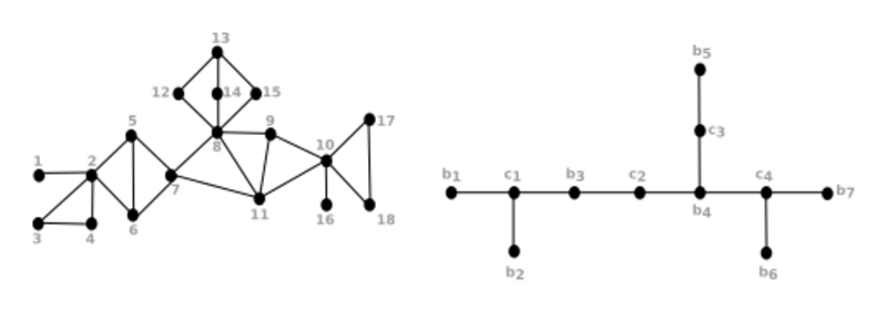
A cutpoint, cut vertex, or articulation point of a graph G is a vertex that is shared by two or more blocks. The structure of the blocks and cutpoints of a connected graph can be described by a tree called the block-cut tree or BC-tree. This tree has a vertex for each block and for each articulation point of the given graph. There is an edge in the block-cut tree for each pair of a block and an articulation point that belongs to that block.

A graph, and its block-cut tree.
Blocks:
b₁ = [1,2]
b₂ = [2,3,4]
b₃ = [2,5,6,7]
b₄ = [7,8,9,10,11]
b₅ = [8,12,13,14,15]
b₆ = [10,16]
b₇ = [10,17,18]
Cutpoints:
c₁ = 2
c₂ = 7
c₃ = 8
c₄ = 10

See also

• Triconnected component
• Bridge (graph theory)
• Single-entry single-exit Counter part of biconnected components in directed graphs

References

• Eugene C. Freuder (1985). "A Sufficient Condition for Backtrack-Bounded Search". Journal of the Association for Computing Machinery 32 (4): 755–761. 

External links

• C++ implementation of Biconnected Components