Biology:Bayesian model of computational anatomy
A major contributor to this article appears to have a close connection with its subject. (December 2017) (Learn how and when to remove this template message) |
Computational anatomy (CA) is a discipline within medical imaging focusing on the study of anatomical shape and form at the visible or gross anatomical scale of morphology. The field is broadly defined and includes foundations in anatomy, applied mathematics and pure mathematics, including medical imaging, neuroscience, physics, probability, and statistics. It focuses on the anatomical structures being imaged, rather than the medical imaging devices. The central focus of the sub-field of computational anatomy within medical imaging is mapping information across anatomical coordinate systems most often dense information measured within a magnetic resonance image (MRI). The introduction of flows into CA, which are akin to the equations of motion used in fluid dynamics, exploit the notion that dense coordinates in image analysis follow the Lagrangian and Eulerian equations of motion. In models based on Lagrangian and Eulerian flows of diffeomorphisms, the constraint is associated to topological properties, such as open sets being preserved, coordinates not crossing implying uniqueness and existence of the inverse mapping, and connected sets remaining connected. The use of diffeomorphic methods grew quickly to dominate the field of mapping methods post Christensen's[1] original paper, with fast and symmetric methods becoming available.[2][3]
The main statistical model

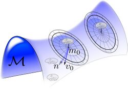
The central statistical model of Computational Anatomy in the context of medical imaging has been the source-channel model of Shannon theory; the source is the deformable template of images , the channel outputs are the imaging sensors with observables (see Figure). The importance of the source-channel model is that the variation in the anatomical configuration are modelled separated from the sensor variations of the Medical imagery. The Bayes theory dictates that the model is characterized by the prior on the source, on , and the conditional density on the observable
conditioned on .
In deformable template theory, the images are linked to the templates, with the deformations a group which acts on the template; see group action in computational anatomy For image action , then the prior on the group induces the prior on images , written as densities the log-posterior takes the form
The random orbit model which follows specifies how to generate the group elements and therefore the random spray of objects which form the prior distribution.
The random orbit model of computational anatomy

The random orbit model of Computational Anatomy first appeared in[4][5][6] modelling the change in coordinates associated to the randomness of the group acting on the templates, which induces the randomness on the source of images in the anatomical orbit of shapes and forms and resulting observations through the medical imaging devices. Such a random orbit model in which randomness on the group induces randomness on the images was examined for the Special Euclidean Group for object recognition in which the group element was the special Euclidean group in.[7]
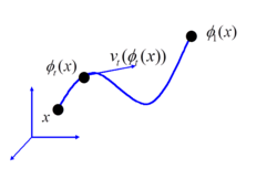
For the study of deformable shape in CA, the high-dimensional diffeomorphism groups used in computational anatomy are generated via smooth flows
which satisfy the Lagrangian and Eulerian specification of the flow fields satisfying the ordinary differential equation:

-
()
with the vector fields on termed the Eulerian velocity of the particles at position of the flow. The vector fields are functions in a function space, modelled as a smooth Hilbert space with the vector fields having 1-continuous derivative . For , the inverse of the flow is given by
-
()
and the Jacobian matrix for flows in given as
To ensure smooth flows of diffeomorphisms with inverse, the vector fields must be at least 1-time continuously differentiable in space[8][9] which are modelled as elements of the Hilbert space using the Sobolev embedding theorems so that each element has 3-square-integrable derivatives. Thus embed smoothly in 1-time continuously differentiable functions.[8][9] The diffeomorphism group are flows with vector fields absolutely integrable in Sobolev norm:
-
()
where with a linear operator defining the norm of the RKHS. The integral is calculated by integration by parts when is a generalized function in the dual space .
Riemannian exponential
In the random orbit model of computational anatomy, the entire flow is reduced to the initial condition which forms the coordinates encoding the diffeomorphism. From the initial condition then geodesic positioning with respect to the Riemannian metric of Computational anatomy solves for the flow of the Euler-Lagrange equation. Solving the geodesic from the initial condition is termed the Riemannian-exponential, a mapping at identity to the group.
The Riemannian exponential satisfies for initial condition , vector field dynamics ,
- for classical equation diffeomorphic shape momentum , , then
- for generalized equation, then ,
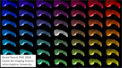
It is extended to the entire group, Depicted in the accompanying figure is a depiction of the random orbits around each exemplar, , generated by randomizing the flow by generating the initial tangent space vector field at the identity , and then generating random object .

Shown in the Figure on the right the cartoon orbit, are a random spray of the subcortical manifolds generated by randomizing the vector fields supported over the submanifolds. The random orbit model induces the prior on shapes and images conditioned on a particular atlas . For this the generative model generates the mean field as a random change in coordinates of the template according to , where the diffeomorphic change in coordinates is generated randomly via the geodesic flows.
MAP estimation in the multiple-atlas orbit model
The random orbit model induces the prior on shapes and images conditioned on a particular atlas . For this the generative model generates the mean field as a random change in coordinates of the template according to , where the diffeomorphic change in coordinates is generated randomly via the geodesic flows. The prior on random transformations on is induced by the flow , with constructed as a Gaussian random field prior . The density on the random observables at the output of the sensor are given by
Maximum a posteriori estimation (MAP) estimation is central to modern statistical theory. Parameters of interest take many forms including (i) disease type such as neurodegenerative or neurodevelopmental diseases, (ii) structure type such as cortical or subcortical structures in problems associated to segmentation of images, and (iii) template reconstruction from populations. Given the observed image , MAP estimation maximizes the posterior:
This requires computation of the conditional probabilities . The multiple atlas orbit model randomizes over the denumerable set of atlases . The model on images in the orbit take the form of a multi-modal mixture distribution
The conditional Gaussian model has been examined heavily for inexact matching in dense images and for landmark matching.
Dense emage matching
Model as a conditionally Gaussian random field conditioned, mean field, . For uniform variance the endpoint error terms plays the role of the log-conditional (only a function of the mean field) giving the endpoint term:
-
()
Landmark matching
Model as conditionally Gaussian with mean field , constant noise variance independent of landmarks. The log-conditional (only a function of the mean field) can be viewed as the endpoint term:
MAP segmentation based on multiple atlases
The random orbit model for multiple atlases models the orbit of shapes as the union over multiple anatomical orbits generated from the group action of diffeomorphisms, , with each atlas having a template and predefined segmentation field . incorporating the parcellation into anatomical structures of the coordinate of the MRI.. The pairs are indexed over the voxel lattice with an MRI image and a dense labelling of every voxel coordinate. The anatomical labelling of parcellated structures are manual delineations by neuroanatomists.
The Bayes segmentation problem[10] is given measurement with mean field and parcellation , the anatomical labelling . mustg be estimated for the measured MRI image. The mean-field of the observable image is modelled as a random deformation from one of the templates , which is also randomly selected, ,. The optimal diffeomorphism is hidden and acts on the background space of coordinates of the randomly selected template image . Given a single atlas , the likelihood model for inference is determined by the joint probability ; with multiple atlases, the fusion of the likelihood functions yields the multi-modal mixture model with the prior averaging over models.
The MAP estimator of segmentation is the maximizer given , which involves the mixture over all atlases.
The quantity is computed via a fusion of likelihoods from multiple deformable atlases, with being the prior probability that the observed image evolves from the specific template image .
The MAP segmentation can be iteratively solved via the expectation–maximization algorithm
MAP estimation of volume templates from populations and the EM algorithm
Generating templates empirically from populations is a fundamental operation ubiquitous to the discipline. Several methods based on Bayesian statistics have emerged for submanifolds and dense image volumes. For the dense image volume case, given the observable the problem is to estimate the template in the orbit of dense images . Ma's procedure takes an initial hypertemplate as the starting point, and models the template in the orbit under the unknown to be estimated diffeomorphism , with the parameters to be estimated the log-coordinates determining the geodesic mapping of the hyper-template .
In the Bayesian random orbit model of computational anatomy the observed MRI images are modelled as a conditionally Gaussian random field with mean field , with a random unknown transformation of the template. The MAP estimation problem is to estimate the unknown template given the observed MRI images.
Ma's procedure for dense imagery takes an initial hypertemplate as the starting point, and models the template in the orbit under the unknown to be estimated diffeomorphism . The observables are modelled as conditional random fields, a conditional-Gaussian random field with mean field . The unknown variable to be estimated explicitly by MAP is the mapping of the hyper-template , with the other mappings considered as nuisance or hidden variables which are integrated out via the Bayes procedure. This is accomplished using the expectation–maximization algorithm.
The orbit-model is exploited by associating the unknown to be estimated flows to their log-coordinates via the Riemannian geodesic log and exponential for computational anatomy the initial vector field in the tangent space at the identity so that , with the mapping of the hyper-template. The MAP estimation problem becomes
The EM algorithm takes as complete data the vector-field coordinates parameterizing the mapping, and compute iteratively the conditional-expectation
- Compute new template maximizing Q-function, setting
- Compute the mode-approximation for the expectation updating the expected-values for the mode values:
References
- ↑ Christensen, G.E.; Rabbitt, R.D.; Miller, M.I. (1996-02-01). "Deformable Templates Using Large Deformation Kinematics". IEEE Transactions on Image Processing 5 (10): 1435–1447. doi:10.1109/83.536892. PMID 18290061. Bibcode: 1996ITIP....5.1435C.
- ↑ Ashburner, J. (July 2007). "A fast diffeomorphic image registration algorithm". NeuroImage 38 (1): 95–113. doi:10.1016/j.neuroimage.2007.07.007. PMID 17761438.
- ↑ Avants, B. B.; Epstein, C. L.; Grossman, M.; Gee, J. C. (2008-02-01). "Symmetric diffeomorphic image registration with cross-correlation: evaluating automated labeling of elderly and neurodegenerative brain". Medical Image Analysis 12 (1): 26–41. doi:10.1016/j.media.2007.06.004. ISSN 1361-8423. PMID 17659998.
- ↑ Miller, Michael; Banerjee, Ayananshu; Christensen, Gary; Joshi, Sarang; Khaneja, Navin; Grenander, Ulf; Matejic, Larissa (1997-06-01). "Statistical methods in computational anatomy". Statistical Methods in Medical Research 6 (3): 267–299. doi:10.1177/096228029700600305. PMID 9339500.
- ↑ U. Grenander and M. I. Miller (2007-02-08). Pattern Theory: From Representation to Inference. Oxford University Press. ISBN 978-0-19-929706-1.
- ↑ M. I. Miller and S. Mori and X. Tang and D. Tward and Y. Zhang (2015-02-14). Bayesian Multiple Atlas Deformable Templates. Brain Mapping: An Encyclopedic Reference. Academic Press. ISBN 978-0-12-397316-0. https://books.google.com/books?id=ysucBAAAQBAJ.
- ↑ Srivastava, S.; Miller, M. I.; Grenander, U. (1997-01-01). Byrnes, Christopher I.. ed. Ergodic Algorithms on Special Euclidean Groups for ATR. Systems & Control: Foundations & Applications. Birkhäuser Boston. pp. 327–350. doi:10.1007/978-1-4612-4120-1_18. ISBN 978-1-4612-8662-2.
- ↑ 8.0 8.1 P. Dupuis, U. Grenander, M.I. Miller, Existence of Solutions on Flows of Diffeomorphisms, Quarterly of Applied Math, 1997.
- ↑ 9.0 9.1 Trouvé, A. (1995). "Action de groupe de dimension infinie et reconnaissance de formes" (in fr). Comptes Rendus de l'Académie des Sciences, Série I 321 (8): 1031–1034.
- ↑ Tang, Xiaoying; Oishi, Kenichi; Faria, Andreia V.; Hillis, Argye E.; Albert, Marilyn S.; Mori, Susumu; Miller, Michael I. (2013-06-18). "Bayesian Parameter Estimation and Segmentation in the Multi-Atlas Random Orbit Model". PLOS ONE 8 (6). doi:10.1371/journal.pone.0065591. PMID 23824159. Bibcode: 2013PLoSO...865591T.
 |
