Biology:Computational anatomy

Short description: Interdisciplinary field of biology

Computational anatomy is an interdisciplinary field of biology focused on quantitative investigation and modelling of anatomical shapes variability. It involves the development and application of mathematical, statistical and data-analytical methods for modelling and simulation of biological structures.

The field is broadly defined and includes foundations in anatomy, applied mathematics and pure mathematics, machine learning, computational mechanics, computational science, biological imaging, neuroscience, physics, probability, and statistics; it also has strong connections with fluid mechanics and geometric mechanics. Additionally, it complements newer, interdisciplinary fields like bioinformatics and neuroinformatics in the sense that its interpretation uses metadata derived from the original sensor imaging modalities (of which magnetic resonance imaging is one example). It focuses on the anatomical structures being imaged, rather than the medical imaging devices. It is similar in spirit to the history of computational linguistics, a discipline that focuses on the linguistic structures rather than the sensor acting as the transmission and communication media.

In computational anatomy, the diffeomorphism group is used to study different coordinate systems via coordinate transformations as generated via the Lagrangian and Eulerian velocities of flow in [math]\displaystyle{ {\mathbb R}^3 }[/math]. The flows between coordinates in computational anatomy are constrained to be geodesic flows satisfying the principle of least action for the Kinetic energy of the flow. The kinetic energy is defined through a Sobolev smoothness norm with strictly more than two generalized, square-integrable derivatives for each component of the flow velocity, which guarantees that the flows in [math]\displaystyle{ \mathbb{R}^3 }[/math] are diffeomorphisms. It also implies that the diffeomorphic shape momentum taken pointwise satisfying the Euler-Lagrange equation for geodesics is determined by its neighbors through spatial derivatives on the velocity field. This separates the discipline from the case of incompressible fluids for which momentum is a pointwise function of velocity. Computational anatomy intersects the study of Riemannian manifolds and nonlinear global analysis, where groups of diffeomorphisms are the central focus. Emerging high-dimensional theories of shape are central to many studies in computational anatomy, as are questions emerging from the fledgling field of shape statistics. The metric structures in computational anatomy are related in spirit to morphometrics, with the distinction that Computational anatomy focuses on an infinite-dimensional space of coordinate systems transformed by a diffeomorphism, hence the central use of the terminology diffeomorphometry, the metric space study of coordinate systems via diffeomorphisms.

Genesis

At computational anatomy's heart is the comparison of shape by recognizing in one shape the other. This connects it to D'Arcy Wentworth Thompson's developments On Growth and Form which has led to scientific explanations of morphogenesis, the process by which patterns are formed in biology. Albrecht Durer's Four Books on Human Proportion were arguably the earliest works on computational anatomy. The efforts of Noam Chomsky in his pioneering of computational linguistics inspired the original formulation of computational anatomy as a generative model of shape and form from exemplars acted upon via transformations.

Due to the availability of dense 3D measurements via technologies such as magnetic resonance imaging (MRI), computational anatomy has emerged as a subfield of medical imaging and bioengineering for extracting anatomical coordinate systems at the morphome scale in 3D. The spirit of this discipline shares strong overlap with areas such as computer vision and kinematics of rigid bodies, where objects are studied by analysing the groups responsible for the movement in question. Computational anatomy departs from computer vision with its focus on rigid motions, as the infinite-dimensional diffeomorphism group is central to the analysis of Biological shapes. It is a branch of the image analysis and pattern theory school at Brown University pioneered by Ulf Grenander. In Grenander's general metric pattern theory, making spaces of patterns into a metric space is one of the fundamental operations since being able to cluster and recognize anatomical configurations often requires a metric of close and far between shapes. The diffeomorphometry metric of computational anatomy measures how far two diffeomorphic changes of coordinates are from each other, which in turn induces a metric on the shapes and images indexed to them. The models of metric pattern theory, in particular group action on the orbit of shapes and forms is a central tool to the formal definitions in computational anatomy.

History

Computational anatomy is the study of shape and form at the morphome or gross anatomy millimeter, or morphology scale, focusing on the study of sub-manifolds of [math]\displaystyle{ {\mathbb R}^3, }[/math] points, curves surfaces and subvolumes of human anatomy. An early modern computational neuro-anatomist was David Van Essen performing some of the early physical unfoldings of the human brain based on printing of a human cortex and cutting. Jean Talairach's publication of Talairach coordinates is an important milestone at the morphome scale demonstrating the fundamental basis of local coordinate systems in studying neuroanatomy and therefore the clear link to charts of differential geometry. Concurrently, virtual mapping in computational anatomy across high resolution dense image coordinates was already happening in Ruzena Bajcy's and Fred Bookstein's earliest developments based on computed axial tomography and magnetic resonance imagery. The earliest introduction of the use of flows of diffeomorphisms for transformation of coordinate systems in image analysis and medical imaging was by Christensen, Joshi, Miller, and Rabbitt.

The first formalization of computational anatomy as an orbit of exemplar templates under diffeomorphism group action was in the original lecture given by Grenander and Miller with that title in May 1997 at the 50th Anniversary of the Division of Applied Mathematics at Brown University, and subsequent publication. This was the basis for the strong departure from much of the previous work on advanced methods for spatial normalization and image registration which were historically built on notions of addition and basis expansion. The structure preserving transformations central to the modern field of Computational Anatomy, homeomorphisms and diffeomorphisms carry smooth submanifolds smoothly. They are generated via Lagrangian and Eulerian flows which satisfy a law of composition of functions forming the group property, but are not additive.

The original model of computational anatomy was as the triple, [math]\displaystyle{ (\mathcal{G}, \mathcal{M}, \mathcal{P}) \ , }[/math] the group [math]\displaystyle{ g \in \mathcal{G} }[/math], the orbit of shapes and forms [math]\displaystyle{ m \in \mathcal{M} }[/math], and the probability laws [math]\displaystyle{ P }[/math] which encode the variations of the objects in the orbit. The template or collection of templates are elements in the orbit [math]\displaystyle{ m_\mathrm{temp} \in \mathcal {M} }[/math] of shapes.

The Lagrangian and Hamiltonian formulations of the equations of motion of computational anatomy took off post 1997 with several pivotal meetings including the 1997 Luminy meeting organized by the Azencott school at Ecole-Normale Cachan on the "Mathematics of Shape Recognition" and the 1998 Trimestre at Institute Henri Poincaré organized by David Mumford "Questions Mathématiques en Traitement du Signal et de l'Image" which catalyzed the Hopkins-Brown-ENS Cachan groups and subsequent developments and connections of computational anatomy to developments in global analysis.

The developments in computational anatomy included the establishment of the Sobolev smoothness conditions on the diffeomorphometry metric to insure existence of solutions of variational problems in the space of diffeomorphisms, the derivation of the Euler-Lagrange equations characterizing geodesics through the group and associated conservation laws, the demonstration of the metric properties of the right invariant metric, the demonstration that the Euler-Lagrange equations have a well-posed initial value problem with unique solutions for all time, and with the first results on sectional curvatures for the diffeomorphometry metric in landmarked spaces. Following the Los Alamos meeting in 2002, Joshi's original large deformation singular Landmark solutions in computational anatomy were connected to peaked solitons or peakons as solutions for the Camassa-Holm equation. Subsequently, connections were made between computational anatomy's Euler-Lagrange equations for momentum densities for the right-invariant metric satisfying Sobolev smoothness to Vladimir Arnold's characterization of the Euler equation for incompressible flows as describing geodesics in the group of volume preserving diffeomorphisms. The first algorithms, generally termed LDDMM for large deformation diffeomorphic mapping for computing connections between landmarks in volumes and spherical manifolds, curves, currents and surfaces, volumes, tensors, varifolds, and time-series have followed.

These contributions of computational anatomy to the global analysis associated to the infinite dimensional manifolds of subgroups of the diffeomorphism group is far from trivial. The original idea of doing differential geometry, curvature and geodesics on infinite dimensional manifolds goes back to Bernhard Riemann's Habilitation (Ueber die Hypothesen, welche der Geometrie zu Grunde liegen); the key modern book laying the foundations of such ideas in global analysis are from Michor.

The applications within medical imaging of computational anatomy continued to flourish after two organized meetings at the Institute for Pure and Applied Mathematics conferences at University of California, Los Angeles. Computational anatomy has been useful in creating accurate models of the atrophy of the human brain at the morphome scale, as well as Cardiac templates, as well as in modeling biological systems. Since the late 1990s, computational anatomy has become an important part of developing emerging technologies for the field of medical imaging. Digital atlases are a fundamental part of modern Medical-school education and in neuroimaging research at the morphome scale. Atlas based methods and virtual textbooks which accommodate variations as in deformable templates are at the center of many neuro-image analysis platforms including Freesurfer, FSL, MRIStudio, SPM. Diffeomorphic registration, introduced in the 1990s, is now an important player with existing codes bases organized around ANTS, DARTEL, DEMONS, LDDMM, StationaryLDDMM, FastLDDMM, are examples of actively used computational codes for constructing correspondences between coordinate systems based on sparse features and dense images. Voxel-based morphometry is an important technology built on many of these principles.

The deformable template orbit model of computational anatomy

The model of human anatomy is a deformable template, an orbit of exemplars under group action. Deformable template models have been central to Grenander's metric pattern theory, accounting for typicality via templates, and accounting for variability via transformation of the template. An orbit under group action as the representation of the deformable template is a classic formulation from differential geometry. The space of shapes are denoted [math]\displaystyle{ m \in \mathcal {M} }[/math], with the group [math]\displaystyle{ (\mathcal{ G}, \circ ) }[/math] with law of composition [math]\displaystyle{ \circ }[/math]; the action of the group on shapes is denoted [math]\displaystyle{ g \cdot m }[/math], where the action of the group [math]\displaystyle{ g \cdot m \in \mathcal{M}, m \in \mathcal {M} }[/math] is defined to satisfy

[math]\displaystyle{ (g \circ g^\prime) \cdot m=g \cdot (g^\prime \cdot m)\in \mathcal { M} . }[/math]

The orbit [math]\displaystyle{ \mathcal{M} }[/math] of the template becomes the space of all shapes, [math]\displaystyle{ \mathcal{M} \doteq \{ m=g \cdot m_\mathrm{temp}, g \in \mathcal{G} \} }[/math], being homogenous under the action of the elements of [math]\displaystyle{ \mathcal{G} }[/math].

Figure depicting three medial temporal lobe structures amygdala, entorhinal cortex and hippocampus with fiducial landmarks depicted as well embedded in the MRI background.

The orbit model of computational anatomy is an abstract algebra - to be compared to linear algebra - since the groups act nonlinearly on the shapes. This is a generalization of the classical models of linear algebra, in which the set of finite dimensional [math]\displaystyle{ {\mathbb R}^n }[/math] vectors are replaced by the finite-dimensional anatomical submanifolds (points, curves, surfaces and volumes) and images of them, and the [math]\displaystyle{ n \times n }[/math] matrices of linear algebra are replaced by coordinate transformations based on linear and affine groups and the more general high-dimensional diffeomorphism groups.

Shapes and forms

The central objects are shapes or forms in computational anatomy, one set of examples being the 0,1,2,3-dimensional submanifolds of [math]\displaystyle{ {\mathbb R}^3 }[/math], a second set of examples being images generated via medical imaging such as via magnetic resonance imaging (MRI) and functional magnetic resonance imaging.

Triangulated mesh surfaces depicting subcortical structures amygdala, hippocampus, thalamus, caudate, putamen, ventricles.The shapes are denoted [math]\displaystyle{ m(u), u \in U\subset {\mathbb R}^1 \rightarrow {\mathbb R}^2 }[/math] represented as triangulated meshes.

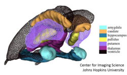
The 0-dimensional manifolds are landmarks or fiducial points; 1-dimensional manifolds are curves such as sulcal and gyral curves in the brain; 2-dimensional manifolds correspond to boundaries of substructures in anatomy such as the subcortical structures of the midbrain or the gyral surface of the neocortex; subvolumes correspond to subregions of the human body, the heart, the thalamus, the kidney.

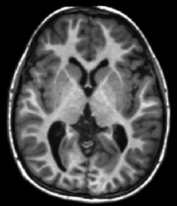
The landmarks [math]\displaystyle{ X \doteq \{ x_1,\dots,x_n \} \subset {\mathbb R}^3 \in \mathcal{M} }[/math] are a collections of points with no other structure, delineating important fiducials within human shape and form (see associated landmarked image). The sub-manifold shapes such as surfaces [math]\displaystyle{ X \subset {\mathbb R}^3 \in \mathcal{M} }[/math] are collections of points modeled as parametrized by a local chart or immersion [math]\displaystyle{ m:U \subset {\mathbb R}^{1,2} \rightarrow {\mathbb R}^3 }[/math], [math]\displaystyle{ m(u), u \in U }[/math] (see Figure showing shapes as mesh surfaces). The images such as MR images or DTI images [math]\displaystyle{ I \in \mathcal{M} }[/math], and are dense functions [math]\displaystyle{ I(x), x \in X \subset {\mathbb R}^{1,2,3} }[/math] are scalars, vectors, and matrices (see Figure showing scalar image).

Groups and group actions

Further information: Group actions in computational anatomy

Showing an MRI section through a 3D brain representing a scalar image [math]\displaystyle{ I(x), x \in {\mathbb R}^2 }[/math] based on T1-weighting.

Groups and group actions are familiar to the Engineering community with the universal popularization and standardization of linear algebra as a basic model for analyzing signals and systems in mechanical engineering, electrical engineering and applied mathematics. In linear algebra the matrix groups (matrices with inverses) are the central structure, with group action defined by the usual definition of [math]\displaystyle{ A }[/math] as an [math]\displaystyle{ n\times n }[/math] matrix, acting on [math]\displaystyle{ x \in {\mathbb R}^n }[/math] as [math]\displaystyle{ n \times 1 }[/math] vectors; the orbit in linear-algebra is the set of [math]\displaystyle{ n }[/math]-vectors given by [math]\displaystyle{ y=A \cdot x \in {\mathbb R}^n }[/math], which is a group action of the matrices through the orbit of [math]\displaystyle{ {\mathbb R}^n }[/math].

The central group in computational anatomy defined on volumes in [math]\displaystyle{ {\mathbb R}^3 }[/math] are the diffeomorphisms [math]\displaystyle{ \mathcal{G} \doteq Diff }[/math] which are mappings with 3-components [math]\displaystyle{ \phi(\cdot)=(\phi_1(\cdot),\phi_2 (\cdot),\phi_3 (\cdot)) }[/math], law of composition of functions [math]\displaystyle{ \phi \circ \phi^\prime (\cdot)\doteq \phi (\phi^\prime(\cdot)) }[/math], with inverse [math]\displaystyle{ \phi \circ \phi^{-1}(\cdot)=\phi ( \phi^{-1}(\cdot))=id }[/math].

Most popular are scalar images, [math]\displaystyle{ I(x),x \in {\mathbb R}^3 }[/math], with action on the right via the inverse.

[math]\displaystyle{ \phi \cdot I(x)=I \circ \phi^{-1} (x), x \in {\mathbb R}^3 }[/math].

For sub-manifolds [math]\displaystyle{ X \subset {\mathbb R}^3 \in \mathcal{M} }[/math], parametrized by a chart or immersion [math]\displaystyle{ m(u), u \in U }[/math], the diffeomorphic action the flow of the position

[math]\displaystyle{ \phi \cdot m(u) \doteq \phi\circ m(u), u \in U }[/math].

Several group actions in computational anatomy have been defined.

Lagrangian and Eulerian flows for generating diffeomorphisms

For the study of rigid body kinematics, the low-dimensional matrix Lie groups have been the central focus. The matrix groups are low-dimensional mappings, which are diffeomorphisms that provide one-to-one correspondences between coordinate systems, with a smooth inverse. The matrix group of rotations and scales can be generated via a closed form finite-dimensional matrices which are solution of simple ordinary differential equations with solutions given by the matrix exponential.

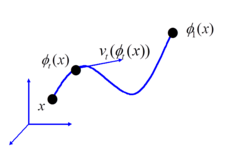
For the study of deformable shape in computational anatomy, a more general diffeomorphism group has been the group of choice, which is the infinite dimensional analogue. The high-dimensional diffeomorphism groups used in Computational Anatomy are generated via smooth flows [math]\displaystyle{ \phi_t, t \in [0,1] }[/math] which satisfy the Lagrangian and Eulerian specification of the flow fields as first introduced in., satisfying the ordinary differential equation:

Showing the Lagrangian flow of coordinates [math]\displaystyle{ x \in X }[/math] with associated vector fields [math]\displaystyle{ v_t, t \in [0,1] }[/math] satisfying ordinary differential equation [math]\displaystyle{ \dot \phi_t=v_t(\phi_t), \phi_0=id }[/math].

[math]\displaystyle{ \frac{d}{dt} \phi_t=v_t \circ \phi_t , \ \phi_0=id \ ; }[/math]

(Lagrangian flow)

with [math]\displaystyle{ v \doteq (v_1,v_2,v_3) }[/math] the vector fields on [math]\displaystyle{ {\mathbb R}^3 }[/math] termed the Eulerian velocity of the particles at position [math]\displaystyle{ \phi }[/math] of the flow. The vector fields are functions in a function space, modelled as a smooth Hilbert space of high-dimension, with the Jacobian of the flow [math]\displaystyle{ \ D\phi \doteq (\frac{\partial \phi_i}{\partial x_j}) }[/math] a high-dimensional field in a function space as well, rather than a low-dimensional matrix as in the matrix groups. Flows were first introduced for large deformations in image matching; [math]\displaystyle{ \dot \phi_t(x) }[/math] is the instantaneous velocity of particle [math]\displaystyle{ x }[/math] at time [math]\displaystyle{ t }[/math] .

The inverse [math]\displaystyle{ \phi_t^{-1}, t \in [0,1] }[/math] required for the group is defined on the Eulerian vector-field with advective inverse flow

[math]\displaystyle{ \frac{d}{dt} \phi_t^{-1}=- (D \phi_t^{-1}) v_t , \ \phi_0^{-1}=id \ . }[/math]

(Inverse Transport flow)

The diffeomorphism group of computational anatomy

The group of diffeomorphisms is very big. To ensure smooth flows of diffeomorphisms avoiding shock-like solutions for the inverse, the vector fields must be at least 1-time continuously differentiable in space. For diffeomorphisms on [math]\displaystyle{ {\mathbb R}^3 }[/math], vector fields are modelled as elements of the Hilbert space [math]\displaystyle{ (V, \|\cdot \|_V ) }[/math] using the Sobolev embedding theorems so that each element has strictly greater than 2 generalized square-integrable spatial derivatives (thus [math]\displaystyle{ v_i \in H_0^3, i=1,2,3, }[/math] is sufficient), yielding 1-time continuously differentiable functions.

The diffeomorphism group are flows with vector fields absolutely integrable in Sobolev norm:

[math]\displaystyle{ Diff_V \doteq \{\varphi=\phi_1: \dot \phi_t=v_t \circ \phi_t , \phi_0=id, \int_0^1 \|v_t \|_V dt \lt \infty \} \ , }[/math]

(Diffeomorphism Group)

where [math]\displaystyle{ \|v\|_V^2 \doteq \int_X Av\cdot v dx, \ v \in V \ , }[/math] with the linear operator [math]\displaystyle{ A }[/math] mapping to the dual space [math]\displaystyle{ A: V \mapsto V^* }[/math], with the integral calculated by integration by parts when [math]\displaystyle{ Av \in V^* }[/math] is a generalized function in the dual space.

Sobolev smoothness and Reproducing Kernel Hilbert Space with Green's kernel

The Sobolev smoothness condition on vector fields as modeled in a reproducing kernel Hilbert space

The modelling approach used in computational anatomy enforces a continuous differentiability condition on the vector fields by modelling the space of vector fields [math]\displaystyle{ (V, \|\cdot \|_V ) }[/math] as a reproducing kernel Hilbert space (RKHS), with the norm defined by a 1-1, differential operator[math]\displaystyle{ A: V \rightarrow V^* }[/math], Green's inverse [math]\displaystyle{ K=A^{-1} }[/math]. The norm of the Hilbert space is induced by the differential operator. For [math]\displaystyle{ \sigma(v) \doteq Av \in V^* }[/math] a generalized function or distribution, define the linear form as [math]\displaystyle{ (\sigma|w)\doteq \int_{{\mathbb R}^3} \sum_i w_i(x) \sigma_i(dx) }[/math]. This determines the norm on [math]\displaystyle{ (V, \|\cdot \|_V ) }[/math] according to

[math]\displaystyle{ \langle v , w \rangle_V \doteq \int_X A v \cdot w dx, \ \|v\|_V^2 \doteq \int_X Av \cdot v dx, \ v,w \in V \ . }[/math]

Since [math]\displaystyle{ A }[/math] is a differential operator, finiteness of the norm-square [math]\displaystyle{ (Av|v) \lt \infty }[/math] includes derivatives from the differential operator implying smoothness of the vector fields.The Sobolev embedding theorem arguments were made in demonstrating that 1-continuous derivative is required for smooth flows. For proper choice of [math]\displaystyle{ A }[/math] then [math]\displaystyle{ (V,\|\cdot \|_V) }[/math] is an RKHS with the operator [math]\displaystyle{ K=A^{-1}: V^* \rightarrow V }[/math] termed the Green's operator generated from the Green's function (scalar case) for the vector field case. The Green's kernels associated to the differential operator smooths since the kernel [math]\displaystyle{ k(\cdot,\cdot) }[/math] is continuously differentiable in both variables implying

[math]\displaystyle{ K\sigma (x)_i \doteq \sum_j \int_{{\mathbb R}^3} k_{ij}(x,y) \sigma_j(dy) }[/math]

When [math]\displaystyle{ \sigma \doteq \mu dx }[/math], a vector density, [math]\displaystyle{ (\sigma|v) \doteq \int v \cdot \mu dx }[/math].

Diffeomorphometry: The metric space of shapes and forms

Further information: Diffeomorphometry

The study of metrics on groups of diffeomorphisms and the study of metrics between manifolds and surfaces has been an area of significant investigation. The diffeomorphometry metric measures how close and far two shapes or images are from each other; the metric length is the shortest length of the flow which carries one coordinate system into the other.

Oftentimes, the familiar Euclidean metric is not directly applicable because the patterns of shapes and images do not form a vector space. In the Riemannian orbit model of computational anatomy, diffeomorphisms acting on the forms [math]\displaystyle{ \phi \cdot m \in \mathcal {M}, \phi \in Diff_V, m \in \mathcal{M} }[/math] do not act linearly. There are many ways to define metrics, and for the sets associated to shapes the Hausdorff metric is another. The method we use to induce the Riemannian metric is used to induce the metric on the orbit of shapes by defining it in terms of the metric length between diffeomorphic coordinate system transformations of the flows. Measuring the lengths of the geodesic flow between coordinates systems in the orbit of shapes is called diffeomorphometry.

The right-invariant metric on diffeomorphisms

Define the distance on the group of diffeomorphisms

[math]\displaystyle{ d_{Diff_V}(\psi, \varphi)=\inf_{v_t} \left(\int_0^1 \int_X Av_t \cdot v_t dx \ dt: \phi_0=\psi, \phi_1=\varphi, \dot \phi_t=v_t \circ \phi_t \right)^{1/2} \ ; }[/math]

(metric-diffeomorphisms)

this is the right-invariant metric of diffeomorphometry, invariant to reparameterization of space since for all [math]\displaystyle{ \phi \in Diff_V }[/math],

[math]\displaystyle{ d_{Diff_V}(\psi, \varphi)=d_{Diff_V}(\psi \circ \phi, \varphi \circ \phi) }[/math].

The metric on shapes and forms

The distance on shapes and forms,[math]\displaystyle{ d_{\mathcal{M}}:\mathcal{M} \times \mathcal{M}\rightarrow \R^+ }[/math],

[math]\displaystyle{ d_{\mathcal{M}}(m,n)=\inf_{\phi \in \operatorname{Diff}_V: \phi \cdot m=n } d_{\operatorname{Diff}_V}(id,\phi) \ ; }[/math]

(metric-shapes-forms)

the images are denoted with the orbit as [math]\displaystyle{ I \in \mathcal{I} }[/math] and metric [math]\displaystyle{ , d_{\mathcal{I}} }[/math].

The action integral for Hamilton's principle on diffeomorphic flows

In classical mechanics the evolution of physical systems is described by solutions to the Euler–Lagrange equations associated to the Least-action principle of Hamilton. This is a standard way, for example of obtaining Newton's laws of motion of free particles. More generally, the Euler-Lagrange equations can be derived for systems of generalized coordinates. The Euler-Lagrange equation in computational anatomy describes the geodesic shortest path flows between coordinate systems of the diffeomorphism metric. In computational anatomy the generalized coordinates are the flow of the diffeomorphism and its Lagrangian velocity [math]\displaystyle{ \phi, \dot{\phi} }[/math], the two related via the Eulerian velocity [math]\displaystyle{ v \doteq \dot{\phi} \circ \phi^{-1} }[/math]. Hamilton's principle for generating the Euler-Lagrange equation requires the action integral on the Lagrangian given by

[math]\displaystyle{ J(\phi) \doteq \int_0^1 L(\phi_t,\dot \phi_t) dt \ ; }[/math]

(Hamiltonian-Integrated-Lagrangian)

the Lagrangian is given by the kinetic energy:

[math]\displaystyle{ L(\phi_t, \dot \phi_t ) \doteq \frac{1}{2} \int_X A (\dot \phi_t \circ \phi_t^{-1}) \cdot (\dot \phi_t \circ \phi_t^{-1} ) dx =\frac{1}{2} \int_X Av_t \cdot v_t \ dx \ . }[/math]

(Lagrangian-Kinetic-Energy)

Diffeomorphic or Eulerian shape momentum

In computational anatomy, [math]\displaystyle{ Av }[/math] was first called the Eulerian or diffeomorphic shape momentum since when integrated against Eulerian velocity [math]\displaystyle{ v }[/math] gives energy density, and since there is a conservation of diffeomorphic shape momentum which holds. The operator [math]\displaystyle{ A }[/math] is the generalized moment of inertia or inertial operator.

The Euler–Lagrange equation on shape momentum for geodesics on the group of diffeomorphisms

Classical calculation of the Euler-Lagrange equation from Hamilton's principle requires the perturbation of the Lagrangian on the vector field in the kinetic energy with respect to first order perturbation of the flow. This requires adjustment by the Lie bracket of vector field, given by operator [math]\displaystyle{ ad_v: w \in V \mapsto V }[/math] which involves the Jacobian given by

[math]\displaystyle{ ad_v[w]\doteq [v,w]\doteq (Dv)w-(Dw)v \in V }[/math].

Defining the adjoint [math]\displaystyle{ ad_v^*: V^* \rightarrow V^*, }[/math] then the first order variation gives the Eulerian shape momentum [math]\displaystyle{ Av \in V^* }[/math] satisfying the generalized equation:

[math]\displaystyle{ \frac{d}{dt} Av_t + ad_{v_t}^* (Av_t)=0 \ , \ t \in [0,1] \  ; }[/math]

(EL-General)

meaning for all smooth [math]\displaystyle{ w \in V , }[/math]

[math]\displaystyle{ \int_X \left( \frac{d}{dt} Av_t + ad_{v_t}^* (Av_t) \right) \cdot w dx=\int_X \frac{d}{dt} Av_t \cdot w dx + \int_X Av_t \cdot ((Dv_t)w-(Dw)v_t) dx=0 . }[/math]

Computational anatomy is the study of the motions of submanifolds, points, curves, surfaces and volumes. Momentum associated to points, curves and surfaces are all singular, implying the momentum is concentrated on subsets of [math]\displaystyle{ {\mathbb R}^3 }[/math] which are dimension [math]\displaystyle{ \leq 2 }[/math] in Lebesgue measure. In such cases, the energy is still well defined [math]\displaystyle{ (Av_t\mid v_t) }[/math] since although [math]\displaystyle{ Av_t }[/math] is a generalized function, the vector fields are smooth and the Eulerian momentum is understood via its action on smooth functions. The perfect illustration of this is even when it is a superposition of delta-diracs, the velocity of the coordinates in the entire volume move smoothly. The Euler-Lagrange equation (EL-General) on diffeomorphisms for generalized functions [math]\displaystyle{ Av \in V^* }[/math] was derived in. In Riemannian Metric and Lie-Bracket Interpretation of the Euler-Lagrange Equation on Geodesics derivations are provided in terms of the adjoint operator and the Lie bracket for the group of diffeomorphisms. It has come to be called EPDiff equation for diffeomorphisms connecting to the Euler-Poincare method having been studied in the context of the inertial operator [math]\displaystyle{ A=identity }[/math] for incompressible, divergence free, fluids.

Diffeomorphic shape momentum: a classical vector function

For the momentum density case [math]\displaystyle{ (Av_t \mid w)=\int_X \mu_t \cdot w \, dx }[/math], then Euler–Lagrange equation has a classical solution:

[math]\displaystyle{ \frac{d}{dt} \mu_t + (Dv_t)^T \mu_t +(D\mu_t)v_t + ( \nabla \cdot v) \mu_t=0 \ , t \in [0,1]. }[/math]

(EL-Classic)

The Euler-Lagrange equation on diffeomorphisms, classically defined for momentum densities first appeared in for medical image analysis.

Riemannian exponential (geodesic positioning) and Riemannian logarithm (geodesic coordinates)

In medical imaging and computational anatomy, positioning and coordinatizing shapes are fundamental operations; the system for positioning anatomical coordinates and shapes built on the metric and the Euler-Lagrange equation a geodesic positioning system as first explicated in Miller Trouve and Younes. Solving the geodesic from the initial condition [math]\displaystyle{ v_0 }[/math] is termed the Riemannian-exponential, a mapping [math]\displaystyle{ Exp_{\rm id}(\cdot): V \to Diff_V }[/math] at identity to the group.

The Riemannian exponential satisfies [math]\displaystyle{ Exp_{id} (v_0)=\phi_1 }[/math] for initial condition [math]\displaystyle{ \dot \phi_0=v_0 }[/math], vector field dynamics [math]\displaystyle{ \dot \phi_t=v_t \circ \phi_t, t \in [0,1] }[/math],

• for classical equation diffeomorphic shape momentum [math]\displaystyle{ \int_X Av_t \cdot w \, dx }[/math], [math]\displaystyle{ Av \in V }[/math], then

[math]\displaystyle{ \ \ \ \frac{d}{dt} Av_t + (Dv_t)^T Av_t +(DAv_t)v_t + ( \nabla \cdot v) Av_t=0 \ ; }[/math]

• for generalized equation, then [math]\displaystyle{ Av \in V^* }[/math],[math]\displaystyle{ w \in V }[/math],

[math]\displaystyle{ \ \ \ \int_X \frac{d}{dt} Av_t \cdot w dx + \int_X Av_t \cdot ((Dv_t)w-(Dw)v_t)dx=0 . }[/math]

Computing the flow [math]\displaystyle{ v_0 }[/math] onto coordinates Riemannian logarithm, mapping [math]\displaystyle{ Log_{\rm id}(\cdot): Diff_V \to V }[/math] at identity from [math]\displaystyle{ \varphi }[/math] to vector field [math]\displaystyle{ v_0 \in V }[/math];

[math]\displaystyle{ Log_{ id}( \varphi)=v_0 \ \text{initial condition of EL geodesic } \dot \phi_0=v_0, \phi_0=id, \phi_1=\varphi \ . }[/math]

Extended to the entire group they become

[math]\displaystyle{ \phi=Exp_\varphi(v_0\circ \varphi) \doteq Exp_{id} (v_0) \circ \varphi }[/math] ; [math]\displaystyle{ Log_\varphi(\phi)\doteq Log_{id}( \phi \circ\varphi^{-1}) \circ \varphi }[/math] .

These are inverses of each other for unique solutions of Logarithm; the first is called geodesic positioning, the latter geodesic coordinates (see exponential map, Riemannian geometry for the finite dimensional version).The geodesic metric is a local flattening of the Riemannian coordinate system (see figure).

Showing metric local flattening of coordinatized manifolds of shapes and forms. The local metric is given by the norm of the vector field [math]\displaystyle{ \|v_0\|_V }[/math] of the geodesic mapping [math]\displaystyle{ Exp_{id}(v_0) \cdot m }[/math]

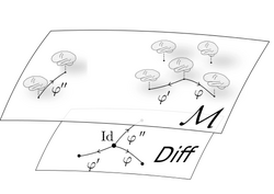
Hamiltonian formulation of computational anatomy

In computational anatomy the diffeomorphisms are used to push the coordinate systems, and the vector fields are used as the control within the anatomical orbit or morphological space. The model is that of a dynamical system, the flow of coordinates [math]\displaystyle{ t \mapsto \phi_t \in \operatorname{Diff}_V }[/math] and the control the vector field [math]\displaystyle{ t \mapsto v_t \in V }[/math] related via [math]\displaystyle{ \dot \phi_t=v_t \cdot \phi_t,\phi_0=id . }[/math] The Hamiltonian view reparameterizes the momentum distribution [math]\displaystyle{ Av \in V^* }[/math] in terms of the conjugate momentum or canonical momentum, introduced as a Lagrange multiplier [math]\displaystyle{ p: \dot \phi \mapsto (p\mid\dot \phi) }[/math] constraining the Lagrangian velocity [math]\displaystyle{ \dot \phi_t=v_t \circ \phi_t }[/math].accordingly:

[math]\displaystyle{ H(\phi_t,p_t,v_t)=\int_X p_t \cdot (v_t \circ \phi_t) dx-\frac{1}{2}\int_X Av_t \cdot v_t dx . }[/math]

This function is the extended Hamiltonian. The Pontryagin maximum principle gives the optimizing vector field which determines the geodesic flow satisfying [math]\displaystyle{ \dot \phi_t=v_t \circ \phi_t , \phi_0=id, }[/math] as well as the reduced Hamiltonian

[math]\displaystyle{ H(\phi_t,p_t) \doteq \max_v H( \phi_t, p_t,v) \ . }[/math]

The Lagrange multiplier in its action as a linear form has its own inner product of the canonical momentum acting on the velocity of the flow which is dependent on the shape, e.g. for landmarks a sum, for surfaces a surface integral, and. for volumes it is a volume integral with respect to [math]\displaystyle{ dx }[/math] on [math]\displaystyle{ {\mathbb R}^3 }[/math]. In all cases the Greens kernels carry weights which are the canonical momentum evolving according to an ordinary differential equation which corresponds to EL but is the geodesic reparameterization in canonical momentum. The optimizing vector field is given by

[math]\displaystyle{ v_t \doteq \arg max_{v} H(\phi_t,p_t,v) }[/math]

with dynamics of canonical momentum reparameterizing the vector field along the geodesic

[math]\displaystyle{ \begin{cases} \dot \phi_t=\frac{\partial H( \phi_t, p_t)}{\partial p} \\ \dot p_t=-\frac{\partial H(\phi_t,p_t)}{\partial \phi} \\ \end{cases} }[/math]

(Hamiltonian-Dynamics)

Stationarity of the Hamiltonian and kinetic energy along Euler–Lagrange

Whereas the vector fields are extended across the entire background space of [math]\displaystyle{ {\mathbb R}^3 }[/math], the geodesic flows associated to the submanifolds has Eulerian shape momentum which evolves as a generalized function [math]\displaystyle{ Av_t \in V^* }[/math] concentrated to the submanifolds. For landmarks the geodesics have Eulerian shape momentum which are a superposition of delta distributions travelling with the finite numbers of particles; the diffeomorphic flow of coordinates have velocities in the range of weighted Green's Kernels. For surfaces, the momentum is a surface integral of delta distributions travelling with the surface.

The geodesics connecting coordinate systems satisfying EL-General have stationarity of the Lagrangian. The Hamiltonian is given by the extremum along the path [math]\displaystyle{ t \in [0,1] }[/math], [math]\displaystyle{ H(\phi,p)=\max_v H(\phi,p,v) }[/math], equalling the Lagrangian-Kinetic-Energy and is stationary along EL-General. Defining the geodesic velocity at the identity [math]\displaystyle{ v_0=\arg \max_v H(\phi_0,p_0,v) }[/math], then along the geodesic

[math]\displaystyle{ H(\phi_t,p_t)=H(\phi_0,p_0)=\frac{1}{2} \int_X p_0 \cdot v_0 dx=\frac{1}{2} \int_X Av_0 \cdot v_0 dx=\frac{1}{2} \int_X Av_t \cdot v_t dx }[/math]

(Hamiltonian-Geodesics)

The stationarity of the Hamiltonian demonstrates the interpretation of the Lagrange multiplier as momentum; integrated against velocity [math]\displaystyle{ \dot \phi }[/math] gives energy density. The canonical momentum has many names. In optimal control, the flows [math]\displaystyle{ \phi }[/math] is interpreted as the state, and [math]\displaystyle{ p }[/math] is interpreted as conjugate state, or conjugate momentum. The geodesi of EL implies specification of the vector fields [math]\displaystyle{ v_0 }[/math] or Eulerian momentum [math]\displaystyle{ Av_0 }[/math] at [math]\displaystyle{ t=0 }[/math], or specification of canonical momentum [math]\displaystyle{ p_0 }[/math] determines the flow.

The metric on geodesic flows of landmarks, surfaces, and volumes within the orbit

In computational anatomy the submanifolds are pointsets, curves, surfaces and subvolumes which are the basic primitives. The geodesic flows between the submanifolds determine the distance, and form the basic measuring and transporting tools of diffeomorphometry. At [math]\displaystyle{ t=0 }[/math] the geodesic has vector field [math]\displaystyle{ v_0=K p_0 }[/math] determined by the conjugate momentum and the Green's kernel of the inertial operator defining the Eulerian momentum [math]\displaystyle{ K=A^{-1} }[/math]. The metric distance between coordinate systems connected via the geodesic determined by the induced distance between identity and group element:

[math]\displaystyle{ d_{Diff_V}(id,\varphi)=\|Log_{id}(\varphi)\|_V=\|v_0 \|_V=\sqrt{2H(id,p_0)} }[/math]

Conservation laws on diffeomorphic shape momentum for computational anatomy

Given the least-action there is a natural definition of momentum associated to generalized coordinates; the quantity acting against velocity gives energy. The field has studied two forms, the momentum associated to the Eulerian vector field termed Eulerian diffeomorphic shape momentum, and the momentum associated to the initial coordinates or canonical coordinates termed canonical diffeomorphic shape momentum. Each has a conservation law. The conservation of momentum goes hand in hand with the EL-General. In computational anatomy, [math]\displaystyle{ Av }[/math] is the Eulerian Momentum since when integrated against Eulerian velocity [math]\displaystyle{ v }[/math] gives energy density; operator [math]\displaystyle{ A }[/math] the generalized moment of inertia or inertial operator which acting on the Eulerian velocity gives momentum which is conserved along the geodesic:

[math]\displaystyle{ \begin{matrix} \text{Eulerian} & \ \ \ \ \frac{d}{dt} \int_X Av_t \cdot ((D \phi_t) w) \circ \phi_t^{-1})dx=0 \ , \ t \in [0,1] . \\ & \\ \text{Canonical} & \ \ \ \ \ \ \ \ \ \ \ \frac{d}{dt} \int_X p_t \cdot ( (D\phi_t) w) dx=0 \ , \ t \in [0,1] \ \text{ for all} \ w \in V \ . \end{matrix} }[/math]

(Euler-Conservation-Constant-Energy)

Conservation of Eulerian shape momentum was shown in and follows from EL-General; conservation of canonical momentum was shown in

Proof of conservation

The proof follow from defining [math]\displaystyle{ w_t=((D \phi_t) w) \circ \phi_t^{-1} }[/math], [math]\displaystyle{ \frac{d}{dt} w_t=(Dv_t) w_t - (D w_t) v_t }[/math] implying [math]\displaystyle{ \frac{d}{dt} (Av_t|((D \phi_t) w) \circ \phi_t^{-1})=(\frac{d}{dt}Av_t|((D \phi_t) w) \circ \phi_t^{-1})+(Av_t|\frac{d}{dt} ((D \phi_t) w) \circ \phi_t^{-1})=(\frac{d}{dt} Av_t|w_t )+(Av_t|(D v_t) w_t-(Dw_t)v_t)=0. }[/math]

The proof on Canonical momentum is shown from [math]\displaystyle{ \dot p_t=- (Dv_t)_{|_{\phi_t}}^T p_t }[/math]:

[math]\displaystyle{ \frac{d}{dt} (p_t|(D\phi_t) w)=(\dot p_t|(D\phi_t) w)+(p_t|\frac{d}{dt} (D\phi_t) w) =(\dot p_t|(D \phi_t) w)+(p_t|(Dv_t)_{|_{\phi_t} }(D \phi_t) w)=0 }[/math].

Geodesic interpolation of information between coordinate systems via variational problems

Further information: Large deformation diffeomorphic metric mapping

Construction of diffeomorphic correspondences between shapes calculates the initial vector field coordinates [math]\displaystyle{ v_0 \in V }[/math] and associated weights on the Greens kernels [math]\displaystyle{ p_0 }[/math]. These initial coordinates are determined by matching of shapes, called Large Deformation Diffeomorphic Metric Mapping (LDDMM). LDDMM has been solved for landmarks with and without correspondence and for dense image matchings. curves, surfaces, dense vector and tensor imagery, and varifolds removing orientation. LDDMM calculates geodesic flows of the EL-General onto target coordinates, adding to the action integral [math]\displaystyle{ \frac{1}{2} \int_0^1 \int_X Av_t\cdot v_t dx dt }[/math] an endpoint matching condition [math]\displaystyle{ E: \phi_1 \rightarrow R^+ }[/math] measuring the correspondence of elements in the orbit under coordinate system transformation. Existence of solutions were examined for image matching. The solution of the variational problem satisfies the EL-General for [math]\displaystyle{ t \in [0,1) }[/math] with boundary condition.

Matching based on minimizing kinetic energy action with endpoint condition

[math]\displaystyle{ \text{min}_{\phi:v=\dot \phi \circ \phi^{-1}, \phi_0=id} C(\phi) \doteq \frac{1}{2} \int_0^1 \int_X Av_t \cdot v_t dx dt +E( \phi_1) }[/math]

[math]\displaystyle{ \begin{cases} \text{Euler Conservation} \ \ \ \ \ \ \ \ & \ \ \ \frac{d}{dt} Av_t + ad_{v_t}^* (Av_t)=0 , \ t \in [0,1) \ , \\ \text{Boundary Condition} & \ \ \ \phi_0=id, Av_1=- \frac{\partial E(\phi)}{\partial \phi}|_{\phi=\phi_1} \ . \end{cases} }[/math]

Conservation from EL-General extends the B.C. at [math]\displaystyle{ t=1 }[/math] to the rest of the path [math]\displaystyle{ t \in [0,1) }[/math]. The inexact matching problem with the endpoint matching term [math]\displaystyle{ E(\phi_1) }[/math] has several alternative forms. One of the key ideas of the stationarity of the Hamiltonian along the geodesic solution is the integrated running cost reduces to initial cost at t=0, geodesics of the EL-General are determined by their initial condition [math]\displaystyle{ v_0 }[/math].

The running cost is reduced to the initial cost determined by [math]\displaystyle{ v_0=Kp_0 }[/math] of Kernel-Surf.-Land.-Geodesics.

Matching based on geodesic shooting

[math]\displaystyle{ \min_{v_0} C(v_0) \doteq \frac{1}{2} \int_X Av_0 \cdot v_0 dx +E(\mathrm{Exp}_\mathrm{id}(v_0) \cdot I_0) \ ; }[/math]

[math]\displaystyle{ \min_{p_0} C(p_0)= \frac{1}{2}\int_X p_0 \cdot Kp_0 dx+ E(\mathrm{Exp}_\text{id}(Kp_0) \cdot I_0) }[/math]

The matching problem explicitly indexed to initial condition [math]\displaystyle{ v_0 }[/math] is called shooting, which can also be reparamerized via the conjugate momentum [math]\displaystyle{ p_0 }[/math].

Dense image matching in computational anatomy

Dense image matching has a long history now with the earliest efforts exploiting a small deformation framework. Large deformations began in the early 1990s, with the first existence to solutions to the variational problem for flows of diffeomorphisms for dense image matching established in. Beg solved via one of the earliest LDDMM algorithms based on solving the variational matching with endpoint defined by the dense imagery with respect to the vector fields, taking variations with respect to the vector fields. Another solution for dense image matching reparameterizes the optimization problem in terms of the state [math]\displaystyle{ q_t \doteq I \circ \phi_t^{-1}, q_0=I }[/math] giving the solution in terms of the infinitesimal action defined by the advection equation.

LDDMM dense image matching

For Beg's LDDMM, denote the Image [math]\displaystyle{ I(x), x \in X }[/math] with group action [math]\displaystyle{ \phi \cdot I \doteq I \circ \phi^{-1} }[/math]. Viewing this as an optimal control problem, the state of the system is the diffeomorphic flow of coordinates [math]\displaystyle{ \phi_t, t \in [0,1] }[/math], with the dynamics relating the control [math]\displaystyle{ v_t, t \in [0,1] }[/math] to the state given by [math]\displaystyle{ \dot \phi=v \circ \phi }[/math]. The endpoint matching condition [math]\displaystyle{ E(\phi_1) \doteq \|I\circ \phi_1^{-1} -I^\prime\|^2 }[/math] gives the variational problem

[math]\displaystyle{ \begin{matrix} & \ \ \ \ \ \min_{v: \dot \phi=v \circ \phi} C(v) \doteq \frac{1}{2} \int_0^1 \int_X Av_t \cdot v_t dx dt +\frac{1}{2} \int_{{\mathbb R}^3}|I\circ \phi_1^{-1}(x)-I^\prime (x)|^2dx \end{matrix} }[/math]

(Dense-Image-Matching)

[math]\displaystyle{ \begin{cases} & \text{Endpoint Condition:} \ \ \ \ \ \ Av_1=\mu_1 dx, \mu_1=(I\circ \phi_1^{-1}-I^\prime ) \nabla (I \circ \phi_1^{-1}) \ ,\\ &\text{Conservation:} \ \ \ \ \ \ \ \ \ \ \ \ \ \ \ Av_t=\mu_t \, dx, \ \mu_t=(D \phi_t^{-1})^T \mu_0 \circ \phi_t^{-1}|D \phi_t^{-1}|\ . \\ & \ \ \ \ \ \ \ \ \ \ \ \ \ \ \ \ \ \ \ \ \ \ \ \ \ \ \ \ \ \ \ \ \ \ \ \ \ \ \ \ \ \ \ \ \ \ \ \ \ \ \ \mu_0=(I - I^\prime \circ \phi_1) \nabla I|D \phi_1|\ . \\ \end{cases} }[/math]

Beg's iterative LDDMM algorithm has fixed points which satisfy the necessary optimizer conditions. The iterative algorithm is given in Beg's LDDMM algorithm for dense image matching.

Hamiltonian LDDMM in the reduced advected state

Denote the Image [math]\displaystyle{ I(x), x \in X }[/math], with state [math]\displaystyle{ q_t \doteq I \circ \phi_t^{-1} }[/math] and the dynamics related state and control given by the advective term [math]\displaystyle{ \dot q_t=- \nabla q_t \cdot v_t }[/math]. The endpoint [math]\displaystyle{ E(q_1) \doteq \|q_1-I^\prime\|^2 }[/math] gives the variational problem

[math]\displaystyle{ \begin{matrix} & \ \ \ \ \ \min_{q: \dot q=v \circ q} C(v) \doteq \frac{1}{2} \int_0^1 \int_X Av_t \cdot v_t dx dt +\frac{1}{2} \int_{{\mathbb R}^3}|q_1(x)-I^\prime(x)|^2dx \end{matrix} }[/math]

(Dense-Image-Matching)

Viallard's iterative Hamiltonian LDDMM has fixed points which satisfy the necessary optimizer conditions.

Diffusion tensor image matching in computational anatomy

Image showing a diffusion tensor image with three color levels depicting the orientations of the three eigenvectors of the matrix image [math]\displaystyle{ I(x), x \in {\mathbb R}^2 }[/math], matrix valued image; each of three colors represents a direction.

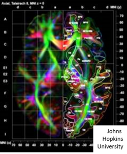
Dense LDDMM tensor matching takes the images as 3x1 vectors and 3x3 tensors solving the variational problem matching between coordinate system based on the principle eigenvectors of the diffusion tensor MRI image (DTI) denoted [math]\displaystyle{ M(x), x \in {\mathbb R}^3 }[/math] consisting of the [math]\displaystyle{ 3 \times 3 }[/math]-tensor at every voxel. Several of the group actions defined based on the Frobenius matrix norm between square matrices [math]\displaystyle{ \|A \|_F^2 \doteq trace A^T A }[/math]. Shown in the accompanying figure is a DTI image illustrated via its color map depicting the eigenvector orientations of the DTI matrix at each voxel with color determined by the orientation of the directions. Denote the [math]\displaystyle{ 3 \times 3 }[/math] tensor image [math]\displaystyle{ M(x), x \in {\mathbb R}^3 }[/math] with eigen-elements [math]\displaystyle{ \{\lambda_i(x), e_i(x), i=1,2,3\} }[/math], [math]\displaystyle{ \lambda_1 \geq \lambda_2 \geq \lambda_3 }[/math].

Coordinate system transformation based on DTI imaging has exploited two actions one based on the principle eigen-vector or entire matrix.

LDDMM matching based on the principal eigenvector of the diffusion tensor matrix takes the image [math]\displaystyle{ I(x), x \in {\mathbb R}^3 }[/math] as a unit vector field defined by the first eigenvector. The group action becomes

[math]\displaystyle{ \varphi \cdot I= \begin{cases} \frac{D_{\varphi^{-1}} \varphi I \circ \varphi^{-1} \|I \circ \varphi^{-1}\|}{\|D_{\varphi^{-1}} \varphi I \circ \varphi^{-1}\|} & I\circ \varphi \neq 0; \\ 0 & \text{otherwise.} \end{cases} }[/math]

LDDMM matching based on the entire tensor matrix has group action becomes [math]\displaystyle{ \varphi \cdot M=(\lambda_1 \hat{e}_1 \hat{e}_1^{T}+\lambda_2 \hat{e}_2 \hat{e}_2^{T} +\lambda_3 \hat{e}_3 \hat{e}_3^{T}) \circ \varphi^{-1} , }[/math] transformed eigenvectors

[math]\displaystyle{ \begin{align} \hat{e}_1 &=\frac{D \varphi e_1}{\|D \varphi e_1\|} \ , \ \ \ \hat{e}_2=\frac{D \varphi e_2-\langle \hat{e}_1,D \varphi e_2\rangle \hat{e}_1}{\sqrt{\|D \varphi e_2\|^2-\langle \hat{e}_1,D \varphi e_2\rangle^2}}\ , \ \ \ \hat{e}_3=\hat{e}_1 \times \hat{e}_2 \end{align} }[/math].

The variational problem matching onto the principal eigenvector or the matrix is described LDDMM Tensor Image Matching.

High Angular Resolution Diffusion Image (HARDI) matching in computational anatomy

High angular resolution diffusion imaging (HARDI) addresses the well-known limitation of DTI, that is, DTI can only reveal one dominant fiber orientation at each location. HARDI measures diffusion along [math]\displaystyle{ n }[/math] uniformly distributed directions on the sphere and can characterize more complex fiber geometries. HARDI can be used to reconstruct an orientation distribution function (ODF) that characterizes the angular profile of the diffusion probability density function of water molecules. The ODF is a function defined on a unit sphere, [math]\displaystyle{ {\mathbb{S}}^2 }[/math].

Dense LDDMM ODF matching takes the HARDI data as ODF at each voxel and solves the LDDMM variational problem in the space of ODF. In the field of information geometry, the space of ODF forms a Riemannian manifold with the Fisher-Rao metric. For the purpose of LDDMM ODF mapping, the square-root representation is chosen because it is one of the most efficient representations found to date as the various Riemannian operations, such as geodesics, exponential maps, and logarithm maps, are available in closed form. In the following, denote square-root ODF ([math]\displaystyle{ {\sqrt{\text{ODF}}} }[/math]) as [math]\displaystyle{ \psi({\bf s}) }[/math], where [math]\displaystyle{ \psi({\bf s}) }[/math] is non-negative to ensure uniqueness and [math]\displaystyle{ \int_{{\bf s}\in {\mathbb{S}}^2} \psi^2({\bf s}) d{\bf s}=1 }[/math]. The variational problem for matching assumes that two ODF volumes can be generated from one to another via flows of diffeomorphisms [math]\displaystyle{ \phi_t }[/math], which are solutions of ordinary differential equations [math]\displaystyle{ \dot \phi_t=v_t (\phi_t), t \in [0,1], }[/math] starting from the identity map [math]\displaystyle{ \phi_0={id} }[/math]. Denote the action of the diffeomorphism on template as [math]\displaystyle{ \phi_1 \cdot \psi_{\mathrm{temp}}({\bf s},x) }[/math], [math]\displaystyle{ {\bf s} \in {{\mathbb{S}}^2} }[/math], [math]\displaystyle{ x \in X }[/math] are respectively the coordinates of the unit sphere, [math]\displaystyle{ {{\mathbb{S}}^2} }[/math] and the image domain, with the target indexed similarly, [math]\displaystyle{ \psi_{\mathrm{targ}}({\bf s}, x) }[/math],[math]\displaystyle{ {\bf s} \in {{\mathbb{S}}^2} }[/math],[math]\displaystyle{ x \in X }[/math].

The group action of the diffeomorphism on the template is given according to

[math]\displaystyle{ \phi_1 \cdot \psi (x)\doteq (D\phi_1) \psi \circ \phi_1^{-1}(x), x \in X }[/math],

where [math]\displaystyle{ (D\phi_1) }[/math] is the Jacobian of the affined transformed ODF and is defined as [math]\displaystyle{ \begin{align} (D \phi_1) \psi\circ \phi_1^{-1}(x)=\sqrt{\frac{\det{\bigl(D_{\phi_1^{-1}}\phi_1 \bigr)^{-1}} }{\left\|{\bigl(D_{\phi_1^{-1}}\phi_1 \bigr)^{-1} } {\bf s} \right\|^3} } \quad \psi \left( \frac{(D_{\phi_1^{-1}}\phi_1 \bigr)^{-1} {\bf s}}{\|(D_{\phi_1^{-1}}\phi_1 \bigr)^{-1} {\bf s}\|}, \phi_1^{-1}(x) \right) . \end{align} }[/math]

This group action of diffeomorphisms on ODF reorients the ODF and reflects changes in both the magnitude of [math]\displaystyle{ \psi }[/math] and the sampling directions of [math]\displaystyle{ \bf s }[/math] due to affine transformation. It guarantees that the volume fraction of fibers oriented toward a small patch must remain the same after the patch is transformed.

The LDDMM variational problem is defined as

[math]\displaystyle{ \begin{align} C(v)=\inf_{v: \dot \phi_t= v_t \circ \phi_t,\phi_0={ id}}\int_0^1 \int_X Av_t \cdot v_t dx \ dt +\lambda \int_{x\in\Omega}\|\log_{(D\phi_1) \psi_{\mathrm{temp}} \circ \phi_1^{-1}(x)}(\psi_{\mathrm{targ}}(x))\|^2_{(D\phi_1) \psi_{\mathrm{temp}}\circ \phi_1^{-1}(x)}dx \end{align} }[/math].

where the logarithm of [math]\displaystyle{ \psi_1, \psi_2 \in \Psi }[/math] is defined as

[math]\displaystyle{ \begin{align} \|\log_{\psi_1}(\psi_2)\|_{\psi_1} =\cos^{-1} \langle \psi_1, \psi_2 \rangle= \cos^{-1}\left(\int_{{\bf s}\in {\mathbb{S}}^2} \psi_1({\bf s}) \psi_2({\bf s})d{\bf s}\right), \end{align} }[/math]

where [math]\displaystyle{ \langle \cdot, \cdot \rangle }[/math] is the normal dot product between points in the sphere under the [math]\displaystyle{ \mathrm{L}^2 }[/math] metric.

This LDDMM-ODF mapping algorithm has been widely used to study brain white matter degeneration in aging, Alzheimer's disease, and vascular dementia. The brain white matter atlas generated based on ODF is constructed via Bayesian estimation. Regression analysis on ODF is developed in the ODF manifold space in.

Metamorphosis

Further information: Biology:Metamorphosis

Demonstrating metamorphosis allowing both diffeomorphic change in coordinate transformation as well as change in image intensity as associated to early Morphing technologies such as the Michael Jackson video. Notice the insertion of tumor gray level intensity which does not exist in template.

The principle mode of variation represented by the orbit model is change of coordinates. For setting in which pairs of images are not related by diffeomorphisms but have photometric variation or image variation not represented by the template, active appearance modelling has been introduced, originally by Edwards-Cootes-Taylor and in 3D medical imaging in. In the context of computational anatomy in which metrics on the anatomical orbit has been studied, metamorphosis for modelling structures such as tumors and photometric changes which are not resident in the template was introduced in for Magnetic Resonance image models, with many subsequent developments extending the metamorphosis framework.

For image matching the image metamorphosis framework enlarges the action so that [math]\displaystyle{ t \mapsto (\phi_t,I_t) }[/math] with action [math]\displaystyle{ \phi_t \cdot I_t \doteq I_t \circ \phi_t^{-1} }[/math]. In this setting metamorphosis combines both the diffeomorphic coordinate system transformation of computational anatomy as well as the early morphing technologies which only faded or modified the photometric or image intensity alone.

Then the matching problem takes a form with equality boundary conditions:

[math]\displaystyle{ \min_{(v,I)} \frac{1}{2} \int_0^1 \left( \int_X A v_t \cdot v_t dx + \|\dot I_t \circ \phi_t^{-1} \|^2 / \sigma^2 \right) \, dt \text{ subject to} \ \phi_0=id, I_0=\text{fixed}, I_1=\text{fixed} }[/math]

Matching landmarks, curves, surfaces

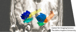
Transforming coordinate systems based on Landmark point or fiducial marker features dates back to Bookstein's early work on small deformation spline methods for interpolating correspondences defined by fiducial points to the two-dimensional or three-dimensional background space in which the fiducials are defined. Large deformation landmark methods came on in the late 1990s. The above Figure depicts a series of landmarks associated three brain structures, the amygdala, entorhinal cortex, and hippocampus.

Matching geometrical objects like unlabelled point distributions, curves or surfaces is another common problem in computational anatomy. Even in the discrete setting where these are commonly given as vertices with meshes, there are no predetermined correspondences between points as opposed to the situation of landmarks described above. From the theoretical point of view, while any submanifold [math]\displaystyle{ X }[/math] in [math]\displaystyle{ {\mathbb R}^3 }[/math], [math]\displaystyle{ d=1,2,3 }[/math] can be parameterized in local charts [math]\displaystyle{ m: u \in U \subset {\mathbb R}^{0,1,2,3} \rightarrow {\mathbb R}^3 }[/math], all reparametrizations of these charts give geometrically the same manifold. Therefore, early on in computational anatomy, investigators have identified the necessity of parametrization invariant representations. One indispensable requirement is that the end-point matching term between two submanifolds is itself independent of their parametrizations. This can be achieved via concepts and methods borrowed from Geometric measure theory, in particular currents and varifolds which have been used extensively for curve and surface matching.

Landmark or point matching with correspondence

Illustration of geodesic flow for one landmark, demonstrating diffeomorphic motion of background space. Red arrow shows [math]\displaystyle{ p_0(1) }[/math], blue curve shows [math]\displaystyle{ \varphi_t(x_1) }[/math], black grid shows [math]\displaystyle{ \varphi_t }[/math]

Figure showing landmark matching with correspondence. Left and right panels depict two different kernel with solutions.

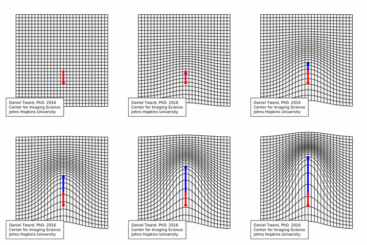
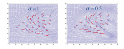
Denoted the landmarked shape [math]\displaystyle{ X\doteq \{ x_1,\dots, x_n \} \subset {\mathbb R}^3 }[/math] with endpoint [math]\displaystyle{ E(\phi_1) \doteq \textstyle \sum_i \displaystyle \|\phi_1(x_i)-x_i^\prime \|^2 }[/math], the variational problem becomes

.[math]\displaystyle{ \begin{matrix} & \ \ \ \min_{\phi: v=\dot \phi \circ \phi^{-1}} C(\phi) \doteq \frac{1}{2} \int (Av_t|v_t)dt +\frac{1}{2} \sum_i \|\phi_1(x_i) - x_i^\prime \|^2 \end{matrix} }[/math]

(Landmark-Matching)

The geodesic Eulerian momentum is a generalized function [math]\displaystyle{ \displaystyle Av_t \in V^*\textstyle, t \in [0,1] }[/math], supported on the landmarked set in the variational problem. The endpoint condition with conservation implies the initial momentum at the identity of the group:

[math]\displaystyle{ \begin{cases} & \text{Endpoint Condition:} \ \ \ \ \ Av_1=\sum_{i=1}^n p_1(i)\delta_{\phi_1(x_i)}, p_1(i)=(x_i^\prime-\phi_1(x_i)) \ , \\ & \text{Conservation:} \ \ \ \ \ \ \ \ \ \ \ \ \ \ Av_t=\sum_{i=1}^n p_t(i) \delta_{\phi_t(x_i)} , \ p_t(i)=(D\phi_{t1})_{|\phi_t(x_i)}^T p_1(i) \ , \ \phi_{t1} \doteq \phi_1 \circ \phi_t^{-1} \ , \\ & \ \ \ \ \ \ \ \ \ \ \ \ \ \ \ \ \ \ \ \ \ \ \ \ \ \ \ \ \ \ \ \ \ \ \ \ \ \ \ \ \ \ \ \ \ Av_0=\sum_i \delta_{x_i} (\cdot) p_0(i) \ \text{with} \ \ p_0(i)=(D\phi_1)^T_{|x_i}(x_i^\prime-\phi_1(x_i)) \end{cases} }[/math]

The iterative algorithm for large deformation diffeomorphic metric mapping for landmarks is given.

Measure matching: unregistered landmarks

Glaunes and co-workers first introduced diffeomorphic matching of pointsets in the general setting of matching distributions. As opposed to landmarks, this includes in particular the situation of weighted point clouds with no predefined correspondences and possibly different cardinalities. The template and target discrete point clouds are represented as two weighted sums of Diracs [math]\displaystyle{ \mu_{m}=\sum_{i=1}^{n} \rho_i \delta_{x_i} }[/math] and [math]\displaystyle{ \mu_{m^\prime}=\sum_{i=1}^{n^\prime} \rho^{\prime}_{i} \delta_{x^{\prime}_{i}} }[/math] living in the space of signed measures of [math]\displaystyle{ \mathbb{R}^3 }[/math]. The space is equipped with a Hilbert metric obtained from a real positive kernel [math]\displaystyle{ k(x,y) }[/math] on [math]\displaystyle{ \mathbb{R}^3 }[/math], giving the following norm:

[math]\displaystyle{ \|\mu_{m} \|_\mathrm{mea}^2=\sum_{i,j=1}^{n} \rho_i \rho_j k(x_i,x_j) }[/math]

The matching problem between a template and target point cloud may be then formulated using this kernel metric for the endpoint matching term:

[math]\displaystyle{ \min_{\phi: v=\dot \phi \circ \phi^{-1}} C(\phi) \doteq \frac{1}{2} \int (Av_t\mid v_t) \, dt +\frac{1}{2} \|\mu_{\phi_1 \cdot m} - \mu_{m^\prime} \|_\mathrm{mea}^2 }[/math]

where [math]\displaystyle{ \mu_{\phi_1 \cdot m}=\sum_{i=1}^{n} \rho_i \delta_{\phi_1(x_i)} }[/math] is the distribution transported by the deformation.

Curve matching

In the one dimensional case, a curve in 3D can be represented by an embedding [math]\displaystyle{ m: u \in [0,1] \rightarrow {\mathbb R}^3 }[/math], and the group action of Diff becomes [math]\displaystyle{ \phi \cdot m=\phi \circ m }[/math]. However, the correspondence between curves and embeddings is not one to one as the any reparametrization [math]\displaystyle{ m \circ \gamma }[/math], for [math]\displaystyle{ \gamma }[/math] a diffeomorphism of the interval [0,1], represents geometrically the same curve. In order to preserve this invariance in the end-point matching term, several extensions of the previous 0-dimensional measure matching approach can be considered.

• Curve matching with currents

In the situation of oriented curves, currents give an efficient setting to construct invariant matching terms. In such representation, curves are interpreted as elements of a functional space dual to the space vector fields, and compared through kernel norms on these spaces. Matching of two curves [math]\displaystyle{ m }[/math] and [math]\displaystyle{ m^\prime }[/math] writes eventually as the variational problem

[math]\displaystyle{ \min_{\phi: v=\dot \phi \circ \phi^{-1}} C(\phi) \doteq \frac{1}{2} \int (Av_t\mid v_t) \, dt +\frac{1}{2} \|\mathcal{C}_{\phi_1 \cdot m} - \mathcal{C}_{m^\prime} \|_\mathrm{cur}^2 }[/math]

with the endpoint term [math]\displaystyle{ E(\phi_1)=\|\mathcal{C}_{\phi_1 \cdot m} - \mathcal{C}_{m^\prime} \|_\mathrm{cur}^2/2 }[/math] is obtained from the norm

[math]\displaystyle{ \|\mathcal{C}_{m} \|_\mathrm{cur}^2=\int_0^1 \int_0^1 K_C(m(u),m(v)) \partial m(u) \cdot \partial m(v) \, du \, dv }[/math]

the derivative [math]\displaystyle{ \partial m(u) }[/math] being the tangent vector to the curve and [math]\displaystyle{ K_{\mathcal{C}} }[/math] a given matrix kernel of [math]\displaystyle{ {\mathbb R}^3 }[/math]. Such expressions are invariant to any positive reparametrizations of [math]\displaystyle{ m }[/math] and [math]\displaystyle{ m' }[/math], and thus still depend on the orientation of the two curves.

• Curve matching with varifolds

Varifold is an alternative to currents when orientation becomes an issue as for instance in situations involving multiple bundles of curves for which no "consistent" orientation may be defined. Varifolds directly extend 0-dimensional measures by adding an extra tangent space direction to the position of points, leading to represent curves as measures on the product of [math]\displaystyle{ {\mathbb R}^3 }[/math] and the Grassmannian of all straight lines in [math]\displaystyle{ {\mathbb R}^3 }[/math]. The matching problem between two curves then consists in replacing the endpoint matching term by [math]\displaystyle{ E(\phi_1)=\|\mathcal{V}_{\phi_1 \cdot m} - \mathcal{V}_{m^\prime} \|_{cur}^2/2 }[/math] with varifold norms of the form:

[math]\displaystyle{ \|\mathcal{V}_m \|_{var}^2=\int_{0}^1 \int_{0}^1 k_{\mathbb{R}^3}(m(u),m(v)) k_{\mathbf{Gr}}\left([\partial m(u)],[\partial m(v)] \right) \partial m(u) {{|}}\partial m(v) {{|}} \, du \, dv }[/math]

where [math]\displaystyle{ [\partial m(u)] }[/math] is the non-oriented line directed by tangent vector [math]\displaystyle{ \partial m(u) }[/math] and [math]\displaystyle{ k_{\mathbb{R}^3}, k_{\mathbf{Gr}} }[/math] two scalar kernels respectively on [math]\displaystyle{ \mathbb{R}^3 }[/math] and the Grassmannian. Due to the inherent non-oriented nature of the Grassmannian representation, such expressions are invariant to positive and negative reparametrizations.

Surface matching

Surface matching share many similarities with the case of curves. Surfaces in [math]\displaystyle{ {\mathbb R}^3 }[/math] are parametrized in local charts by embeddings [math]\displaystyle{ m: u \in U \subset {\mathbb R}^{2} \rightarrow {\mathbb R}^3 }[/math], with all reparametrizations [math]\displaystyle{ m\circ \gamma }[/math] with [math]\displaystyle{ \gamma }[/math] a diffeomorphism of U being equivalent geometrically. Currents and varifolds can be also used to formalize surface matching.

• Surface matching with currents

Oriented surfaces can be represented as 2-currents which are dual to differential 2-forms. In [math]\displaystyle{ {\mathbb R}^3 }[/math], one can further identify 2-forms with vector fields through the standard wedge product of 3D vectors. In that setting, surface matching writes again:

[math]\displaystyle{ \min_{\phi: v=\dot \phi \circ \phi^{-1}} C(\phi) \doteq \frac{1}{2} \int (Av_t\mid v_t) \, dt +\frac{1}{2} \|\mathcal{C}_{\phi_1 \cdot m} - \mathcal{C}_{m^\prime} \|_\mathrm{cur}^2 }[/math]

with the endpoint term [math]\displaystyle{ E(\phi_1)=\|\mathcal{C}_{\phi_1 \cdot m} - \mathcal{C}_{m^\prime} \|_\mathrm{cur}^2/2 }[/math] given through the norm

[math]\displaystyle{ \|\mathcal{C}_{m} \|_\mathrm{cur}^2=\iint_{U\times U} K_C(m(u),m(v)) \vec{n}(u) \cdot \vec{n}(v) \, du \, dv }[/math]

with [math]\displaystyle{ \vec{n}=\partial_{u_1} m \wedge \partial_{u_2} m }[/math] the normal vector to the surface parametrized by [math]\displaystyle{ m }[/math].

This surface mapping algorithm has been validated for brain cortical surfaces against CARET and FreeSurfer. LDDMM mapping for multiscale surfaces is discussed in.

• Surface matching with varifolds

For non-orientable or non-oriented surfaces, the varifold framework is often more adequate. Identifying the parametric surface [math]\displaystyle{ m }[/math] with a varifold [math]\displaystyle{ \mathcal{V}_m }[/math] in the space of measures on the product of [math]\displaystyle{ {\mathbb R}^3 }[/math] and the Grassmannian, one simply replaces the previous current metric [math]\displaystyle{ \|\mathcal{C}_{m} \|_\mathrm{cur}^2 }[/math] by:

[math]\displaystyle{ \|\mathcal{V}_{m} \|_\mathrm{var}^2=\iint_{U\times U} k_{\mathbb{R}^3}(m(u),m(v)) k_{\mathbf{Gr}}\left([\vec{n}(u)],[\vec{n}(v)] \right) {{|}}\vec{n}(u){{|}} {{|}}\vec{n}(v) {{|}} \, du \, dv }[/math]

where [math]\displaystyle{ [\vec{n}(u)] }[/math] is the (non-oriented) line directed by the normal vector to the surface.

Growth and atrophy from longitudinal time-series

There are many settings in which there are a series of measurements, a time-series to which the underlying coordinate systems will be matched and flowed onto. This occurs for example in the dynamic growth and atrophy models and motion tracking such as have been explored in An observed time sequence is given and the goal is to infer the time flow of geometric change of coordinates carrying the exemplars or templars through the period of observations.

The generic time-series matching problem considers the series of times is [math]\displaystyle{ 0 \lt t_1 \lt \dots t_K=1 }[/math]. The flow optimizes at the series of costs [math]\displaystyle{ E(t_k), k=1, \dots, K }[/math] giving optimization problems of the form

[math]\displaystyle{ \min_{\phi:v=\dot \phi \circ \phi^{-1}, \phi_0=id} C(\phi) \doteq \frac{1}{2} \int_0^1 (Av_t\mid v_t) \, dt +\sum_{k=1}^K E( \phi_{t_k}) }[/math].

There have been at least three solutions offered thus far, piecewise geodesic, principal geodesic and splines.

The random orbit model of computational anatomy

Orbits of brains associated to diffeomorphic group action on templates depicted via smooth flow associated to geodesic flows with random spray associated to random generation of initial tangent space vector field [math]\displaystyle{ v_0 \in V }[/math]; published in.

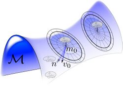
The random orbit model of computational anatomy first appeared in modelling the change in coordinates associated to the randomness of the group acting on the templates, which induces the randomness on the source of images in the anatomical orbit of shapes and forms and resulting observations through the medical imaging devices. Such a random orbit model in which randomness on the group induces randomness on the images was examined for the Special Euclidean Group for object recognition in.

Depicted in the figure is a depiction of the random orbits around each exemplar, [math]\displaystyle{ m_0 \in \mathcal{M} }[/math], generated by randomizing the flow by generating the initial tangent space vector field at the identity [math]\displaystyle{ v_0 \in V }[/math], and then generating random object [math]\displaystyle{ n \doteq Exp_{id}(v_0) \cdot m_0 \in \mathcal{M} }[/math].

The random orbit model induces the prior on shapes and images [math]\displaystyle{ I \in \mathcal{I} }[/math] conditioned on a particular atlas [math]\displaystyle{ I_a \in \mathcal{I} }[/math]. For this the generative model generates the mean field [math]\displaystyle{ I }[/math] as a random change in coordinates of the template according to [math]\displaystyle{ I \doteq \phi \cdot I_a }[/math], where the diffeomorphic change in coordinates is generated randomly via the geodesic flows. The prior on random transformations [math]\displaystyle{ \pi_{Diff} (d\phi) }[/math] on [math]\displaystyle{ Diff_V }[/math] is induced by the flow [math]\displaystyle{ Exp_{id}(v) }[/math], with [math]\displaystyle{ v \in V }[/math] constructed as a Gaussian random field prior [math]\displaystyle{ \pi_V(dv) }[/math]. The density on the random observables at the output of the sensor [math]\displaystyle{ I^D \in \mathcal{I}^D }[/math] are given by

Figure showing the random spray of synthesized subcortical structures laid out in the two-dimensional grid representing the variance of the eigenfunction used for the momentum for synthesis.

[math]\displaystyle{ p(I^D|I_a)=\int_V p(I^D|Exp_{id}(v) \cdot I_a ) \pi_V (dv) \ . }[/math]

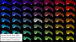
Shown in the Figure on the right the cartoon orbit, are a random spray of the subcortical manifolds generated by randomizing the vector fields [math]\displaystyle{ v_0 }[/math] supported over the submanifolds.

The Bayesian model of computational anatomy

Source-channel model showing the source of images the deformable template [math]\displaystyle{ I \doteq \phi \cdot I_\mathrm{temp} \in \mathcal{I} }[/math] and channel output associated with MRI sensor [math]\displaystyle{ I^D \in \mathcal{I}^{\mathcal{D}} }[/math]

The central statistical model of computational anatomy in the context of medical imaging has been the source-channel model of Shannon theory; the source is the deformable template of images [math]\displaystyle{ I \in \mathcal {I} }[/math], the channel outputs are the imaging sensors with observables [math]\displaystyle{ I^D \in {\mathcal I}^{\mathcal D} }[/math] (see Figure).

See The Bayesian model of computational anatomy for discussions (i) MAP estimation with multiple atlases, (ii) MAP segmentation with multiple atlases, MAP estimation of templates from populations.

Statistical shape theory in computational anatomy

Further information: Statistical shape analysis and Shape theory (mathematics)

Shape in computational anatomy is a local theory, indexing shapes and structures to templates to which they are bijectively mapped. Statistical shape in computational anatomy is the empirical study of diffeomorphic correspondences between populations and common template coordinate systems. This is a strong departure from Procrustes Analyses and shape theories pioneered by David G. Kendall in that the central group of Kendall's theories are the finite-dimensional Lie groups, whereas the theories of shape in computational anatomy have focused on the diffeomorphism group, which to first order via the Jacobian can be thought of as a field–thus infinite dimensional–of low-dimensional Lie groups of scale and rotations.

Figure showing hundreds of sub-cortical structures embedded in two-dimensional momentum space generated from the first two eigenvectors of the empirical co-variance estimated from the population of shapes.

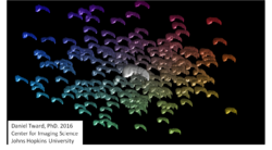
The random orbit model provides the natural setting to understand empirical shape and shape statistics within computational anatomy since the non-linearity of the induced probability law on anatomical shapes and forms [math]\displaystyle{ m \in \mathcal{M} }[/math] is induced via the reduction to the vector fields [math]\displaystyle{ v_0 \in V }[/math] at the tangent space at the identity of the diffeomorphism group. The successive flow of the Euler equation induces the random space of shapes and forms [math]\displaystyle{ Exp_{id}(v_0) \cdot m \in \mathcal{M} }[/math].

Performing empirical statistics on this tangent space at the identity is the natural way for inducing probability laws on the statistics of shape. Since both the vector fields and the Eulerian momentum [math]\displaystyle{ Av_0 }[/math] are in a Hilbert space the natural model is one of a Gaussian random field, so that given test function [math]\displaystyle{ w \in V }[/math], then the inner-products with the test functions are Gaussian distributed with mean and covariance.

This is depicted in the accompanying figure where sub-cortical brain structures are depicted in a two-dimensional coordinate system based on inner products of their initial vector fields that generate them from the template is shown in a 2-dimensional span of the Hilbert space.

Template estimation from populations

Depicting template estimation from multiplie subcortical surfaces in populations of MR images using the EM-algorithm solution of Ma.

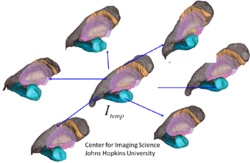
The study of shape and statistics in populations are local theories, indexing shapes and structures to templates to which they are bijectively mapped. Statistical shape is then the study of diffeomorphic correspondences relative to the template. A core operation is the generation of templates from populations, estimating a shape that is matched to the population. There are several important methods for generating templates including methods based on Frechet averaging, and statistical approaches based on the expectation-maximization algorithm and the Bayes Random orbit models of computational anatomy. Shown in the accompanying figure is a subcortical template reconstruction from the population of MRI subjects.

Software for diffeomorphic mapping

Software suites containing a variety of diffeomorphic mapping algorithms include the following:

• ANTS
• DARTEL Voxel-based morphometry
• DEFORMETRICA
• DEMONS
• LDDMM Large deformation diffeomorphic metric mapping
• LDDMM based on frame-based kernel
• StationaryLDDMM

Cloud software

• MRICloud

See also

• Bayesian estimation of templates in computational anatomy
• Computational neuroanatomy
• Geometric data analysis
• Large deformation diffeomorphic metric mapping
• Procrustes analysis
• Riemannian metric and Lie-bracket in computational anatomy
• Shape analysis (disambiguation)
• Statistical shape analysis

References

{{|}}