Borůvka's algorithm

Short description: Method for finding minimum spanning trees

Borůvka's algorithm

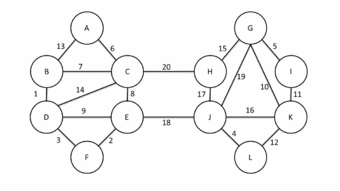
Animation of Borůvka's algorithm
Class	Minimum spanning tree algorithm
Data structure	Graph
Worst-case performance	[math]\displaystyle{ O(|E|\log |V|) }[/math]
Worst-case space complexity	{{{space}}}

Borůvka's algorithm is a greedy algorithm for finding a minimum spanning tree in a graph, or a minimum spanning forest in the case of a graph that is not connected.

It was first published in 1926 by Otakar Borůvka as a method of constructing an efficient electricity network for Moravia. The algorithm was rediscovered by Choquet in 1938; again by Florek, Łukasiewicz, Perkal, Steinhaus, and Zubrzycki in 1951; and again by Georges Sollin in 1965. This algorithm is frequently called Sollin's algorithm, especially in the parallel computing literature.

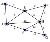
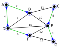
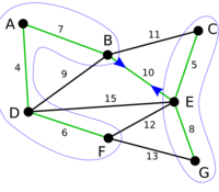
The algorithm begins by finding the minimum-weight edge incident to each vertex of the graph, and adding all of those edges to the forest. Then, it repeats a similar process of finding the minimum-weight edge from each tree constructed so far to a different tree, and adding all of those edges to the forest. Each repetition of this process reduces the number of trees, within each connected component of the graph, to at most half of this former value, so after logarithmically many repetitions the process finishes. When it does, the set of edges it has added forms the minimum spanning forest.

Pseudocode

The following pseudocode illustrates a basic implementation of Borůvka's algorithm. In the conditional clauses, every edge uv is considered cheaper than "None". The purpose of the completed variable is to determine whether the forest F is yet a spanning forest.

If edges do not have distinct weights, then a consistent tie-breaking rule must be used, e.g. based on some total order on vertices or edges. This can be achieved by representing vertices as integers and comparing them directly; comparing their memory addresses; etc. A tie-breaking rule is necessary to ensure that the created graph is indeed a forest, that is, it does not contain cycles. For example, consider a triangle graph with nodes {a,b,c} and all edges of weight 1. Then a cycle could be created if we select ab as the minimal weight edge for {a}, bc for {b}, and ca for {c}. A tie-breaking rule which orders edges first by source, then by destination, will prevent creation of a cycle, resulting in the minimal spanning tree {ab, bc}.

algorithm Borůvka is
    input: A weighted undirected graph G = (V, E).
    output: F, a minimum spanning forest of G.

    Initialize a forest F to (V, E') where E' = {}.

    completed := false
    while not completed do
        Find the connected components of F and assign to each vertex its component
        Initialize the cheapest edge for each component to "None"
        for each edge uv in E, where u and v are in different components of F:
            let wx be the cheapest edge for the component of u
            if is-preferred-over(uv, wx) then
                Set uv as the cheapest edge for the component of u
            let yz be the cheapest edge for the component of v
            if is-preferred-over(uv, yz) then
                Set uv as the cheapest edge for the component of v
        if all components have cheapest edge set to "None" then
            // no more trees can be merged -- we are finished
            completed := true
        else
            completed := false
            for each component whose cheapest edge is not "None" do
                Add its cheapest edge to E'

function is-preferred-over(edge1, edge2) is
    return (edge2 is "None") or
           (weight(edge1) < weight(edge2)) or
           (weight(edge1) = weight(edge2) and tie-breaking-rule(edge1, edge2))

function tie-breaking-rule(edge1, edge2) is
    The tie-breaking rule; returns true if and only if edge1
    is preferred over edge2 in the case of a tie.

As an optimization, one could remove from G each edge that is found to connect two vertices in the same component, so that it does not contribute to the time for searching for cheapest edges in later components.

Complexity

Borůvka's algorithm can be shown to take O(log V) iterations of the outer loop until it terminates, and therefore to run in time O(E log V), where E is the number of edges, and V is the number of vertices in G (assuming E ≥ V). In planar graphs, and more generally in families of graphs closed under graph minor operations, it can be made to run in linear time, by removing all but the cheapest edge between each pair of components after each stage of the algorithm.

Example

Image	components	Description
	{A} {B} {C} {D} {E} {F} {G}	This is our original weighted graph. The numbers near the edges indicate their weight. Initially, every vertex by itself is a component (blue circles).
	{A,B,D,F} {C,E,G}	In the first iteration of the outer loop, the minimum weight edge out of every component is added. Some edges are selected twice (AD, CE). Two components remain.
	{A,B,C,D,E,F,G}	In the second and final iteration, the minimum weight edge out of each of the two remaining components is added. These happen to be the same edge. One component remains and we are done. The edge BD is not considered because both endpoints are in the same component.

Other algorithms

Other algorithms for this problem include Prim's algorithm and Kruskal's algorithm. Fast parallel algorithms can be obtained by combining Prim's algorithm with Borůvka's.

A faster randomized minimum spanning tree algorithm based in part on Borůvka's algorithm due to Karger, Klein, and Tarjan runs in expected O(E) time. The best known (deterministic) minimum spanning tree algorithm by Bernard Chazelle is also based in part on Borůvka's and runs in O(E α(E,V)) time, where α is the inverse Ackermann function. These randomized and deterministic algorithms combine steps of Borůvka's algorithm, reducing the number of components that remain to be connected, with steps of a different type that reduce the number of edges between pairs of components.