Greedy algorithm

Short description: Sequence of locally optimal choices

Greedy algorithms determine the minimum number of coins to give while making change. These are the steps most people would take to emulate a greedy algorithm to represent 36 cents using only coins with values {1, 5, 10, 20}. The coin of the highest value, less than the remaining change owed, is the local optimum. (In general, the change-making problem requires dynamic programming to find an optimal solution; however, most currency systems are special cases where the greedy strategy does find an optimal solution.)

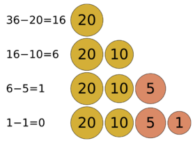
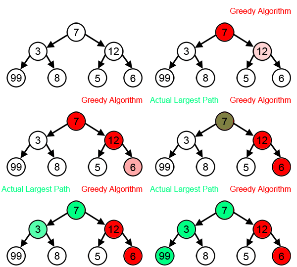
A greedy algorithm is any algorithm that follows the problem-solving heuristic of making the locally optimal choice at each stage. In many problems, a greedy strategy does not produce an optimal solution, but a greedy heuristic can yield locally optimal solutions that approximate a globally optimal solution in a reasonable amount of time.

For example, a greedy strategy for the travelling salesman problem (which is of high computational complexity) is the following heuristic: "At each step of the journey, visit the nearest unvisited city." This heuristic does not intend to find the best solution, but it terminates in a reasonable number of steps; finding an optimal solution to such a complex problem typically requires unreasonably many steps. In mathematical optimization, greedy algorithms optimally solve combinatorial problems having the properties of matroids and give constant-factor approximations to optimization problems with the submodular structure.

Specifics

Greedy algorithms produce good solutions on some mathematical problems, but not on others. Most problems for which they work will have two properties:

Greedy choice property

We can make whatever choice seems best at the moment and then solve the subproblems that arise later. The choice made by a greedy algorithm may depend on choices made so far, but not on future choices or all the solutions to the subproblem. It iteratively makes one greedy choice after another, reducing each given problem into a smaller one. In other words, a greedy algorithm never reconsiders its choices. This is the main difference from dynamic programming, which is exhaustive and is guaranteed to find the solution. After every stage, dynamic programming makes decisions based on all the decisions made in the previous stage and may reconsider the previous stage's algorithmic path to the solution.

Optimal substructure

"A problem exhibits optimal substructure if an optimal solution to the problem contains optimal solutions to the sub-problems."

Cases of failure

Examples on how a greedy algorithm may fail to achieve the optimal solution.

Starting from A, a greedy algorithm that tries to find the maximum by following the greatest slope will find the local maximum at "m", oblivious to the global maximum at "M".

To reach the largest sum, at each step, the greedy algorithm will choose what appears to be the optimal immediate choice, so it will choose 12 instead of 3 at the second step, and will not reach the best solution, which contains 99.

Greedy algorithms fail to produce the optimal solution for many other problems and may even produce the unique worst possible solution. One example is the travelling salesman problem mentioned above: for each number of cities, there is an assignment of distances between the cities for which the nearest-neighbour heuristic produces the unique worst possible tour. For other possible examples, see horizon effect.

Types

Greedy algorithms can be characterized as being 'short sighted', and also as 'non-recoverable'. They are ideal only for problems that have an 'optimal substructure'. Despite this, for many simple problems, the best-suited algorithms are greedy. It is important, however, to note that the greedy algorithm can be used as a selection algorithm to prioritize options within a search, or branch-and-bound algorithm. There are a few variations to the greedy algorithm:

• Pure greedy algorithms
• Orthogonal greedy algorithms
• Relaxed greedy algorithms

Theory

Greedy algorithms have a long history of study in combinatorial optimization and theoretical computer science. Greedy heuristics are known to produce suboptimal results on many problems, and so natural questions are:

• For which problems do greedy algorithms perform optimally?
• For which problems do greedy algorithms guarantee an approximately optimal solution?
• For which problems are the greedy algorithm guaranteed not to produce an optimal solution?

A large body of literature exists answering these questions for general classes of problems, such as matroids, as well as for specific problems, such as set cover.

Matroids

A matroid is a mathematical structure that generalizes the notion of linear independence from vector spaces to arbitrary sets. If an optimization problem has the structure of a matroid, then the appropriate greedy algorithm will solve it optimally.

Submodular functions

A function [math]\displaystyle{ f }[/math] defined on subsets of a set [math]\displaystyle{ \Omega }[/math] is called submodular if for every [math]\displaystyle{ S, T \subseteq \Omega }[/math] we have that [math]\displaystyle{ f(S)+f(T)\geq f(S\cup T)+f(S\cap T) }[/math].

Suppose one wants to find a set [math]\displaystyle{ S }[/math] which maximizes [math]\displaystyle{ f }[/math]. The greedy algorithm, which builds up a set [math]\displaystyle{ S }[/math] by incrementally adding the element which increases [math]\displaystyle{ f }[/math] the most at each step, produces as output a set that is at least [math]\displaystyle{ (1 - 1/e) \max_{X \subseteq \Omega} f(X) }[/math]. That is, greedy performs within a constant factor of [math]\displaystyle{ (1 - 1/e) \approx 0.63 }[/math] as good as the optimal solution.

Similar guarantees are provable when additional constraints, such as cardinality constraints, are imposed on the output, though often slight variations on the greedy algorithm are required. See for an overview.

Other problems with guarantees

Other problems for which the greedy algorithm gives a strong guarantee, but not an optimal solution, include

• Set cover
• The Steiner tree problem
• Load balancing
• Independent set

Many of these problems have matching lower bounds; i.e., the greedy algorithm does not perform better than the guarantee in the worst case.

Applications

Greedy algorithms typically (but not always) fail to find the globally optimal solution because they usually do not operate exhaustively on all the data. They can make commitments to certain choices too early, preventing them from finding the best overall solution later. For example, all known greedy coloring algorithms for the graph coloring problem and all other NP-complete problems do not consistently find optimum solutions. Nevertheless, they are useful because they are quick to think up and often give good approximations to the optimum.

If a greedy algorithm can be proven to yield the global optimum for a given problem class, it typically becomes the method of choice because it is faster than other optimization methods like dynamic programming. Examples of such greedy algorithms are Kruskal's algorithm and Prim's algorithm for finding minimum spanning trees and the algorithm for finding optimum Huffman trees.

Greedy algorithms appear in the network routing as well. Using greedy routing, a message is forwarded to the neighbouring node which is "closest" to the destination. The notion of a node's location (and hence "closeness") may be determined by its physical location, as in geographic routing used by ad hoc networks. Location may also be an entirely artificial construct as in small world routing and distributed hash table.

Examples

• The activity selection problem is characteristic of this class of problems, where the goal is to pick the maximum number of activities that do not clash with each other.
• In the Macintosh computer game Crystal Quest the objective is to collect crystals, in a fashion similar to the travelling salesman problem. The game has a demo mode, where the game uses a greedy algorithm to go to every crystal. The artificial intelligence does not account for obstacles, so the demo mode often ends quickly.
• The matching pursuit is an example of a greedy algorithm applied on signal approximation.
• A greedy algorithm finds the optimal solution to Malfatti's problem of finding three disjoint circles within a given triangle that maximize the total area of the circles; it is conjectured that the same greedy algorithm is optimal for any number of circles.
• A greedy algorithm is used to construct a Huffman tree during Huffman coding where it finds an optimal solution.
• In decision tree learning, greedy algorithms are commonly used, however they are not guaranteed to find the optimal solution.
  • One popular such algorithm is the ID3 algorithm for decision tree construction.
• Dijkstra's algorithm and the related A* search algorithm are verifiably optimal greedy algorithms for graph search and shortest path finding.
  • A* search is conditionally optimal, requiring an "admissible heuristic" that will not overestimate path costs.
• Kruskal's algorithm and Prim's algorithm are greedy algorithms for constructing minimum spanning trees of a given connected graph. They always find an optimal solution, which may not be unique in general.
• The Sequitur and Lempel-Ziv-Welch algorithms are greedy algorithms for grammar induction.

See also

• Best-first search
• Epsilon-greedy strategy
• Greedy algorithm for Egyptian fractions
• Greedy source
• Hill climbing
• Horizon effect
• Matroid

References

Sources

• Cormen, Thomas H.; Leiserson, Charles E.; Rivest, Ronald L.; Stein, Clifford (2001). "16 Greedy Algorithms". Introduction To Algorithms. MIT Press. pp. 370–. ISBN 978-0-262-03293-3. https://books.google.com/books?id=NLngYyWFl_YC&pg=PA370. 
• Gutin, Gregory; Yeo, Anders; Zverovich, Alexey (2002). "Traveling salesman should not be greedy: Domination analysis of greedy-type heuristics for the TSP". Discrete Applied Mathematics 117 (1–3): 81–86. doi:10.1016/S0166-218X(01)00195-0. 
• Bang-Jensen, Jørgen; Gutin, Gregory; Yeo, Anders (2004). "When the greedy algorithm fails". Discrete Optimization 1 (2): 121–127. doi:10.1016/j.disopt.2004.03.007. 
• Bendall, Gareth; Margot, François (2006). "Greedy-type resistance of combinatorial problems". Discrete Optimization 3 (4): 288–298. doi:10.1016/j.disopt.2006.03.001. 
• Feige, U. (1998). "A threshold of ln n for approximating set cover". Journal of the ACM 45 (4): 634–652. doi:10.1145/285055.285059. https://www.cs.duke.edu/courses/cps296.2/spring07/papers/p634-feige.pdf. 
• Nemhauser, G.; Wolsey, L.A.; Fisher, M.L. (1978). "An analysis of approximations for maximizing submodular set functions—I". Mathematical Programming 14 (1): 265–294. doi:10.1007/BF01588971. https://www.researchgate.net/publication/242914003. 
• Buchbinder, Niv; Feldman, Moran; Naor, Joseph (Seffi); Schwartz, Roy (2014). "Submodular maximization with cardinality constraints". Proceedings of the twenty-fifth annual ACM-SIAM symposium on Discrete algorithms. Society for Industrial and Applied Mathematics. doi:10.1137/1.9781611973402.106. ISBN 978-1-61197-340-2. http://theory.epfl.ch/moranfe/Publications/SODA2014.pdf. 
• Krause, A.; Golovin, D. (2014). "Submodular Function Maximization". in Bordeaux, L.; Hamadi, Y.; Kohli, P.. Tractability: Practical Approaches to Hard Problems. Cambridge University Press. pp. 71–104. doi:10.1017/CBO9781139177801.004. ISBN 9781139177801. https://books.google.com/books?id=YxliAgAAQBAJ&pg=PA71. 
• Papadimitriou, Christos H.; Steiglitz, Kenneth (1998). Combinatorial Optimization: Algorithms and Complexity. Dover. 

External links

• Hazewinkel, Michiel, ed. (2001), "Greedy algorithm", Encyclopedia of Mathematics, Springer Science+Business Media B.V. / Kluwer Academic Publishers, ISBN 978-1-55608-010-4, https://www.encyclopediaofmath.org/index.php?title=p/g110210 
• Gift, Noah. "Python greedy coin example". http://www.oreillynet.com/onlamp/blog/2008/04/python_greedy_coin_changer_alg.html.

References

- ↑ Black, Paul E. (2 February 2005). "greedy algorithm". Dictionary of Algorithms and Data Structures. U.S. National Institute of Standards and Technology (NIST). http://xlinux.nist.gov/dads//HTML/greedyalgo.html.
- ↑ van Melkebeek, Dieter. "Greedy Approximations". https://pages.cs.wisc.edu/~dieter/Courses/2004F-CS787/Scribes/greedy-approx.pdf.
- ↑ Frieze, Alan; Pegden, Wesley (2023-10-05). "The bright side of simple heuristics for the TSP". arXiv:2310.03222 [cs.DM].
- ↑ Cormen et al. 2001, Ch. 16
- ↑ Erickson, Jeff (2019). "Greedy Algorithms". Algorithms. University of Illinois at Urbana-Champaign. https://jeffe.cs.illinois.edu/teaching/algorithms/.