Data validation and reconciliation

Short description: A technology to correct measurements in industrial processes

Industrial process data validation and reconciliation, or more briefly, process data reconciliation (PDR), is a technology that uses process information and mathematical methods in order to automatically ensure data validation and reconciliation by correcting measurements in industrial processes. The use of PDR allows for extracting accurate and reliable information about the state of industry processes from raw measurement data and produces a single consistent set of data representing the most likely process operation.

Models, data and measurement errors

Industrial processes, for example chemical or thermodynamic processes in chemical plants, refineries, oil or gas production sites, or power plants, are often represented by two fundamental means:

1. Models that express the general structure of the processes,
2. Data that reflects the state of the processes at a given point in time.

Models can have different levels of detail, for example one can incorporate simple mass or compound conservation balances, or more advanced thermodynamic models including energy conservation laws. Mathematically the model can be expressed by a nonlinear system of equations [math]\displaystyle{ F(y)=0\, }[/math] in the variables [math]\displaystyle{ y=(y_1,\ldots,y_n) }[/math], which incorporates all the above-mentioned system constraints (for example the mass or heat balances around a unit). A variable could be the temperature or the pressure at a certain place in the plant.

Error types

• Random and systematic errors
• 

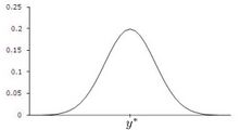  Normally distributed measurements without bias.

• 

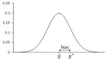  Normally distributed measurements with bias.

Data originates typically from measurements taken at different places throughout the industrial site, for example temperature, pressure, volumetric flow rate measurements etc. To understand the basic principles of PDR, it is important to first recognize that plant measurements are never 100% correct, i.e. raw measurement [math]\displaystyle{ y\, }[/math] is not a solution of the nonlinear system [math]\displaystyle{ F(y)=0\,\! }[/math]. When using measurements without correction to generate plant balances, it is common to have incoherencies. Measurement errors can be categorized into two basic types:

1. random errors due to intrinsic sensor accuracy and
2. systematic errors (or gross errors) due to sensor calibration or faulty data transmission.

Random errors means that the measurement [math]\displaystyle{ y\,\! }[/math] is a random variable with mean [math]\displaystyle{ y^*\,\! }[/math], where [math]\displaystyle{ y^*\,\! }[/math] is the true value that is typically not known. A systematic error on the other hand is characterized by a measurement [math]\displaystyle{ y\,\! }[/math] which is a random variable with mean [math]\displaystyle{ \bar{y}\,\! }[/math], which is not equal to the true value [math]\displaystyle{ y^*\, }[/math]. For ease in deriving and implementing an optimal estimation solution, and based on arguments that errors are the sum of many factors (so that the Central limit theorem has some effect), data reconciliation assumes these errors are normally distributed.

Other sources of errors when calculating plant balances include process faults such as leaks, unmodeled heat losses, incorrect physical properties or other physical parameters used in equations, and incorrect structure such as unmodeled bypass lines. Other errors include unmodeled plant dynamics such as holdup changes, and other instabilities in plant operations that violate steady state (algebraic) models. Additional dynamic errors arise when measurements and samples are not taken at the same time, especially lab analyses.

The normal practice of using time averages for the data input partly reduces the dynamic problems. However, that does not completely resolve timing inconsistencies for infrequently-sampled data like lab analyses.

This use of average values, like a moving average, acts as a low-pass filter, so high frequency noise is mostly eliminated. The result is that, in practice, data reconciliation is mainly making adjustments to correct systematic errors like biases.

Necessity of removing measurement errors

ISA-95 is the international standard for the integration of enterprise and control systems It asserts that:

Data reconciliation is a serious issue for enterprise-control integration. The data have to be valid to be useful for the enterprise system. The data must often be determined from physical measurements that have associated error factors. This must usually be converted into exact values for the enterprise system. This conversion may require manual, or intelligent reconciliation of the converted values [...]. Systems must be set up to ensure that accurate data are sent to production and from production. Inadvertent operator or clerical errors may result in too much production, too little production, the wrong production, incorrect inventory, or missing inventory.

History

PDR has become more and more important due to industrial processes that are becoming more and more complex. PDR started in the early 1960s with applications aiming at closing material balances in production processes where raw measurements were available for all variables. At the same time the problem of gross error identification and elimination has been presented. In the late 1960s and 1970s unmeasured variables were taken into account in the data reconciliation process., PDR also became more mature by considering general nonlinear equation systems coming from thermodynamic models., , Quasi steady state dynamics for filtering and simultaneous parameter estimation over time were introduced in 1977 by Stanley and Mah. Dynamic PDR was formulated as a nonlinear optimization problem by Liebman et al. in 1992.

Data reconciliation

Data reconciliation is a technique that targets at correcting measurement errors that are due to measurement noise, i.e. random errors. From a statistical point of view the main assumption is that no systematic errors exist in the set of measurements, since they may bias the reconciliation results and reduce the robustness of the reconciliation.

Given [math]\displaystyle{ n }[/math] measurements [math]\displaystyle{ y_i }[/math], data reconciliation can mathematically be expressed as an optimization problem of the following form:

[math]\displaystyle{ \begin{align} \min_{x,y^*} & \sum_{i=1}^n\left(\frac{y_i^*-y_i}{\sigma_i}\right)^2 \\ \text{subject to } & F(x,y^*)=0 \\ & y_\min \le y^*\le y_\max\\ & x_\min \le x\le x_\max, \end{align}\,\! }[/math]

where [math]\displaystyle{ y_i^*\,\! }[/math] is the reconciled value of the [math]\displaystyle{ i }[/math]-th measurement ([math]\displaystyle{ i=1,\ldots,n\,\! }[/math]), [math]\displaystyle{ y_i\,\! }[/math] is the measured value of the [math]\displaystyle{ i }[/math]-th measurement ([math]\displaystyle{ i=1,\ldots,n\,\! }[/math]), [math]\displaystyle{ x_j\,\! }[/math] is the [math]\displaystyle{ j }[/math]-th unmeasured variable ([math]\displaystyle{ j=1,\ldots,m\,\! }[/math]), and [math]\displaystyle{ \sigma_i\,\! }[/math] is the standard deviation of the [math]\displaystyle{ i }[/math]-th measurement ([math]\displaystyle{ i=1,\ldots,n\,\! }[/math]), [math]\displaystyle{ F(x,y^*)=0\,\! }[/math] are the [math]\displaystyle{ p\,\! }[/math] process equality constraints and [math]\displaystyle{ x_{\min}, x_{\max}, y_{\min}, y_{\max}\,\! }[/math] are the bounds on the measured and unmeasured variables.

The term [math]\displaystyle{ \left(\frac{y_i^*-y_i}{\sigma_i}\right)^2\,\! }[/math] is called the penalty of measurement i. The objective function is the sum of the penalties, which will be denoted in the following by [math]\displaystyle{ f(y^*)=\sum_{i=1}^n\left(\frac{y_i^*-y_i}{\sigma_i}\right)^2 }[/math].

In other words, one wants to minimize the overall correction (measured in the least squares term) that is needed in order to satisfy the system constraints. Additionally, each least squares term is weighted by the standard deviation of the corresponding measurement. The standard deviation is related to the accuracy of the measurement. For example, at a 95% confidence level, the standard deviation is about half the accuracy.

Redundancy

• Sensor and topological redundancy
• 

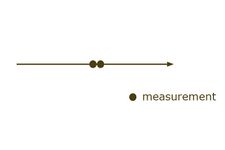  Sensor redundancy arising from multiple sensors of the same quantity at the same time at the same place.

• 

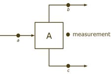  Topological redundancy arising from model information, using the mass conservation constraint [math]\displaystyle{ a=b+c\,\! }[/math], for example one can calculate [math]\displaystyle{ c\,\! }[/math], when [math]\displaystyle{ a\,\! }[/math] and [math]\displaystyle{ b\,\! }[/math] are known.

Data reconciliation relies strongly on the concept of redundancy to correct the measurements as little as possible in order to satisfy the process constraints. Here, redundancy is defined differently from redundancy in information theory. Instead, redundancy arises from combining sensor data with the model (algebraic constraints), sometimes more specifically called "spatial redundancy", "analytical redundancy", or "topological redundancy".

Redundancy can be due to sensor redundancy, where sensors are duplicated in order to have more than one measurement of the same quantity. Redundancy also arises when a single variable can be estimated in several independent ways from separate sets of measurements at a given time or time averaging period, using the algebraic constraints.

Redundancy is linked to the concept of observability. A variable (or system) is observable if the models and sensor measurements can be used to uniquely determine its value (system state). A sensor is redundant if its removal causes no loss of observability. Rigorous definitions of observability, calculability, and redundancy, along with criteria for determining it, were established by Stanley and Mah, for these cases with set constraints such as algebraic equations and inequalities. Next, we illustrate some special cases:

Topological redundancy is intimately linked with the degrees of freedom ([math]\displaystyle{ dof\,\! }[/math]) of a mathematical system, i.e. the minimum number of pieces of information (i.e. measurements) that are required in order to calculate all of the system variables. For instance, in the example above the flow conservation requires that [math]\displaystyle{ a=b+c\, }[/math]. One needs to know the value of two of the 3 variables in order to calculate the third one. The degrees of freedom for the model in that case is equal to 2. At least 2 measurements are needed to estimate all the variables, and 3 would be needed for redundancy.

When speaking about topological redundancy we have to distinguish between measured and unmeasured variables. In the following let us denote by [math]\displaystyle{ x\,\! }[/math] the unmeasured variables and [math]\displaystyle{ y\,\! }[/math] the measured variables. Then the system of the process constraints becomes [math]\displaystyle{ F(x,y)=0\,\! }[/math], which is a nonlinear system in [math]\displaystyle{ y\,\! }[/math] and [math]\displaystyle{ x\,\! }[/math]. If the system [math]\displaystyle{ F(x,y)=0\,\! }[/math] is calculable with the [math]\displaystyle{ n\, }[/math] measurements given, then the level of topological redundancy is defined as [math]\displaystyle{ red= n - dof\,\! }[/math], i.e. the number of additional measurements that are at hand on top of those measurements which are required in order to just calculate the system. Another way of viewing the level of redundancy is to use the definition of [math]\displaystyle{ dof\, }[/math], which is the difference between the number of variables (measured and unmeasured) and the number of equations. Then one gets

[math]\displaystyle{ \begin{align} red= n - dof = n-(n+m-p) = p-m, \end{align} }[/math]

i.e. the redundancy is the difference between the number of equations [math]\displaystyle{ p\, }[/math] and the number of unmeasured variables [math]\displaystyle{ m\, }[/math]. The level of total redundancy is the sum of sensor redundancy and topological redundancy. We speak of positive redundancy if the system is calculable and the total redundancy is positive. One can see that the level of topological redundancy merely depends on the number of equations (the more equations the higher the redundancy) and the number of unmeasured variables (the more unmeasured variables, the lower the redundancy) and not on the number of measured variables.

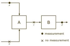
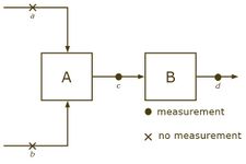
Simple counts of variables, equations, and measurements are inadequate for many systems, breaking down for several reasons: (a) Portions of a system might have redundancy, while others do not, and some portions might not even be possible to calculate, and (b) Nonlinearities can lead to different conclusions at different operating points. As an example, consider the following system with 4 streams and 2 units.

Example of calculable and non-calculable systems

• Calculable and non-calculable systems
• 

  Calculable system, from [math]\displaystyle{ d\,\! }[/math] one can compute [math]\displaystyle{ c\,\! }[/math], and knowing [math]\displaystyle{ a\,\! }[/math] yields [math]\displaystyle{ b\,\! }[/math].

• 

  non-calculable system, knowing [math]\displaystyle{ c\,\! }[/math] does not give information about [math]\displaystyle{ a\,\! }[/math] and [math]\displaystyle{ b\,\! }[/math].

We incorporate only flow conservation constraints and obtain [math]\displaystyle{ a+b=c\,\! }[/math] and [math]\displaystyle{ c=d\,\! }[/math]. It is possible that the system [math]\displaystyle{ F(x,y)=0\,\! }[/math] is not calculable, even though [math]\displaystyle{ p-m\ge 0\,\! }[/math].

If we have measurements for [math]\displaystyle{ c\,\! }[/math] and [math]\displaystyle{ d\,\! }[/math], but not for [math]\displaystyle{ a\,\! }[/math] and [math]\displaystyle{ b\,\! }[/math], then the system cannot be calculated (knowing [math]\displaystyle{ c\,\! }[/math] does not give information about [math]\displaystyle{ a\,\! }[/math] and [math]\displaystyle{ b\,\! }[/math]). On the other hand, if [math]\displaystyle{ a\,\! }[/math] and [math]\displaystyle{ d\,\! }[/math] are known, but not [math]\displaystyle{ b\,\! }[/math] and [math]\displaystyle{ c\,\! }[/math], then the system can be calculated.

In 1981, observability and redundancy criteria were proven for these sorts of flow networks involving only mass and energy balance constraints. After combining all the plant inputs and outputs into an "environment node", loss of observability corresponds to cycles of unmeasured streams. That is seen in the second case above, where streams a and b are in a cycle of unmeasured streams. Redundancy classification follows, by testing for a path of unmeasured streams, since that would lead to an unmeasured cycle if the measurement was removed. Measurements c and d are redundant in the second case above, even though part of the system is unobservable.

Benefits

Redundancy can be used as a source of information to cross-check and correct the measurements [math]\displaystyle{ y\,\! }[/math] and increase their accuracy and precision: on the one hand they reconciled Further, the data reconciliation problem presented above also includes unmeasured variables [math]\displaystyle{ x\,\! }[/math]. Based on information redundancy, estimates for these unmeasured variables can be calculated along with their accuracies. In industrial processes these unmeasured variables that data reconciliation provides are referred to as soft sensors or virtual sensors, where hardware sensors are not installed.

Data validation

Data validation denotes all validation and verification actions before and after the reconciliation step.

Data filtering

Data filtering denotes the process of treating measured data such that the values become meaningful and lie within the range of expected values. Data filtering is necessary before the reconciliation process in order to increase robustness of the reconciliation step. There are several ways of data filtering, for example taking the average of several measured values over a well-defined time period.

Result validation

Result validation is the set of validation or verification actions taken after the reconciliation process and it takes into account measured and unmeasured variables as well as reconciled values. Result validation covers, but is not limited to, penalty analysis for determining the reliability of the reconciliation, or bound checks to ensure that the reconciled values lie in a certain range, e.g. the temperature has to be within some reasonable bounds.

Gross error detection

Result validation may include statistical tests to validate the reliability of the reconciled values, by checking whether gross errors exist in the set of measured values. These tests can be for example

• the chi square test (global test)
• the individual test.

If no gross errors exist in the set of measured values, then each penalty term in the objective function is a random variable that is normally distributed with mean equal to 0 and variance equal to 1. By consequence, the objective function is a random variable which follows a chi-square distribution, since it is the sum of the square of normally distributed random variables. Comparing the value of the objective function [math]\displaystyle{ f(y^*)\,\! }[/math] with a given percentile [math]\displaystyle{ P_{\alpha}\, }[/math] of the probability density function of a chi-square distribution (e.g. the 95th percentile for a 95% confidence) gives an indication of whether a gross error exists: If [math]\displaystyle{ f(y^*)\le P_{95} }[/math], then no gross errors exist with 95% probability. The chi square test gives only a rough indication about the existence of gross errors, and it is easy to conduct: one only has to compare the value of the objective function with the critical value of the chi square distribution.

The individual test compares each penalty term in the objective function with the critical values of the normal distribution. If the [math]\displaystyle{ i }[/math]-th penalty term is outside the 95% confidence interval of the normal distribution, then there is reason to believe that this measurement has a gross error.

Advanced process data reconciliation

Advanced process data reconciliation (PDR) is an integrated approach of combining data reconciliation and data validation techniques, which is characterized by

• complex models incorporating besides mass balances also thermodynamics, momentum balances, equilibria constraints, hydrodynamics etc.
• gross error remediation techniques to ensure meaningfulness of the reconciled values,
• robust algorithms for solving the reconciliation problem.

Thermodynamic models

Simple models include mass balances only. When adding thermodynamic constraints such as energy balances to the model, its scope and the level of redundancy increases. Indeed, as we have seen above, the level of redundancy is defined as [math]\displaystyle{ p-m }[/math], where [math]\displaystyle{ p }[/math] is the number of equations. Including energy balances means adding equations to the system, which results in a higher level of redundancy (provided that enough measurements are available, or equivalently, not too many variables are unmeasured).

Gross error remediation

thumb|350px|The workflow of an advanced data validation and reconciliation process. Gross errors are measurement systematic errors that may bias the reconciliation results. Therefore, it is important to identify and eliminate these gross errors from the reconciliation process. After the reconciliation statistical tests can be applied that indicate whether or not a gross error does exist somewhere in the set of measurements. These techniques of gross error remediation are based on two concepts:

• gross error elimination
• gross error relaxation.

Gross error elimination determines one measurement that is biased by a systematic error and discards this measurement from the data set. The determination of the measurement to be discarded is based on different kinds of penalty terms that express how much the measured values deviate from the reconciled values. Once the gross errors are detected they are discarded from the measurements and the reconciliation can be done without these faulty measurements that spoil the reconciliation process. If needed, the elimination is repeated until no gross error exists in the set of measurements.

Gross error relaxation targets at relaxing the estimate for the uncertainty of suspicious measurements so that the reconciled value is in the 95% confidence interval. Relaxation typically finds application when it is not possible to determine which measurement around one unit is responsible for the gross error (equivalence of gross errors). Then measurement uncertainties of the measurements involved are increased.

It is important to note that the remediation of gross errors reduces the quality of the reconciliation, either the redundancy decreases (elimination) or the uncertainty of the measured data increases (relaxation). Therefore, it can only be applied when the initial level of redundancy is high enough to ensure that the data reconciliation can still be done (see Section 2,).

Workflow

Advanced PDR solutions offer an integration of the techniques mentioned above:

1. data acquisition from data historian, data base or manual inputs
2. data validation and filtering of raw measurements
3. data reconciliation of filtered measurements
4. result verification
   • range check
   • gross error remediation (and go back to step 3)
5. result storage (raw measurements together with reconciled values)

The result of an advanced PDR procedure is a coherent set of validated and reconciled process data.

Applications

PDR finds application mainly in industry sectors where either measurements are not accurate or even non-existing, like for example in the upstream sector where flow meters are difficult or expensive to position (see ); or where accurate data is of high importance, for example for security reasons in nuclear power plants (see ). Another field of application is performance and process monitoring (see ) in oil refining or in the chemical industry.

As PDR enables to calculate estimates even for unmeasured variables in a reliable way, the German Engineering Society (VDI Gesellschaft Energie und Umwelt) has accepted the technology of PDR as a means to replace expensive sensors in the nuclear power industry (see VDI norm 2048,).

See also

• Process simulation
• Pinch analysis
• Industrial processes
• Chemical engineering

References

• Alexander, Dave, Tannar, Dave & Wasik, Larry "Mill Information System uses Dynamic Data Reconciliation for Accurate Energy Accounting" TAPPI Fall Conference 2007.[1]
• Rankin, J. & Wasik, L. "Dynamic Data Reconciliation of Batch Pulping Processes (for On-Line Prediction)" PAPTAC Spring Conference 2009.
• S. Narasimhan, C. Jordache, Data reconciliation and gross error detection: an intelligent use of process data, Golf Publishing Company, Houston, 2000.
• V. Veverka, F. Madron, 'Material and Energy Balancing in the Process Industries, Elsevier Science BV, Amsterdam, 1997.
• J. Romagnoli, M.C. Sanchez, Data processing and reconciliation for chemical process operations, Academic Press, 2000.

References

- ↑ "ISA-95: the international standard for the integration of enterprise and control systems". isa-95.com.
- ↑ D.R. Kuehn, H. Davidson, Computer Control II. Mathematics of Control, Chem. Eng. Process 57: 44–47, 1961.
- ↑ V. Vaclavek, Studies on System Engineering I. On the Application of the Calculus of the Observations of Calculations of Chemical Engineering Balances, Coll. Czech Chem. Commun. 34: 3653, 1968.
- ↑ V. Vaclavek, M. Loucka, Selection of Measurements Necessary to Achieve Multicomponent Mass Balances in Chemical Plant, Chem. Eng. Sci. 31: 1199–1205, 1976.
- ↑ R.S.H. Mah, G.M. Stanley, D.W. Downing, Reconciliation and Rectification of Process Flow and Inventory Data, Ind. & Eng. Chem. Proc. Des. Dev. 15: 175–183, 1976.
- ↑ J.C. Knepper, J.W. Gorman, Statistical Analysis of Constrained Data Sets, AiChE Journal 26: 260–164, 1961.
- ↑ 7.0 7.1 7.2 G.M. Stanley and R.S.H. Mah, Estimation of Flows and Temperatures in Process Networks, AIChE Journal 23: 642–650, 1977.
- ↑ P. Joris, B. Kalitventzeff, Process measurements analysis and validation, Proc. CEF’87: Use Comput. Chem. Eng., Italy, 41–46, 1987.
- ↑ M.J. Liebman, T.F. Edgar, L.S. Lasdon, Efficient Data Reconciliation and Estimation for Dynamic Processes Using Nonlinear Programming Techniques, Computers Chem. Eng. 16: 963–986, 1992.
- ↑ Stanley G.M. and Mah, R.S.H., "Observability and Redundancy in Process Data Estimation, Chem. Engng. Sci. 36, 259 (1981)
- ↑ 11.0 11.1 11.2 VDI-Gesellschaft Energie und Umwelt, "Guidelines - VDI 2048 Blatt 1 - “Control and quality improvement of process data and their uncertainties by means of correction calculation for operation and acceptance tests”; VDI 2048 Part 1; September 2017", Association of German Engineers, 2017.
- ↑ Stanley G.M., and Mah R.S.H., "Observability and Redundancy Classification in Process Networks", Chem. Engng. Sci. 36, 1941 (1981)
- ↑ P. Delava, E. Maréchal, B. Vrielynck, B. Kalitventzeff (1999), Modelling of a Crude Oil Distillation Unit in Term of Data Reconciliation with ASTM or TBP Curves as Direct Input – Application : Crude Oil Preheating Train, Proceedings of ESCAPE-9 conference, Budapest, May 31-June 2, 1999, supplementary volume, p. 17-20.
- ↑ M. Langenstein, J. Jansky, B. Laipple (2004), Finding Megawatts in nuclear power plants with process data validation, Proceedings of ICONE12, Arlington, USA, April 25–29, 2004.
- ↑ Th. Amand, G. Heyen, B. Kalitventzeff, Plant Monitoring and Fault Detection: Synergy between Data Reconciliation and Principal Component Analysis, Comp. and Chem, Eng. 25, p. 501-507, 2001.