Earth:Geodesic grid
_illustrated.png)
A geodesic grid is a spatial grid based on a geodesic polyhedron or Goldberg polyhedron.
History
The earliest use of the (icosahedral) geodesic grid in geophysical modeling dates back to 1968 and the work by Sadourny, Arakawa, and Mintz[1] and Williamson.[2][3] Later work expanded on this base.[4][5][6][7][8]
Construction
A geodesic grid is a global Earth spatial reference that uses polygon tiles based on the subdivision of a polyhedron (usually the icosahedron, and usually a Class I subdivision) to subdivide the surface of the Earth. Such a grid does not have a straightforward relationship to latitude and longitude, but conforms to many of the main criteria for a statistically valid discrete global grid.[9] Primarily, the cells' area and shape are generally similar, especially near the poles where many other spatial grids have singularities or heavy distortion. The popular Quaternary Triangular Mesh (QTM) falls into this category.[10]
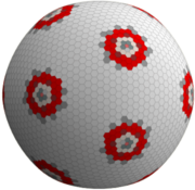
Geodesic grids may use the dual polyhedron of the geodesic polyhedron, which is the Goldberg polyhedron. Goldberg polyhedra are made up of hexagons and (if based on the icosahedron) 12 pentagons. One implementation that uses an icosahedron as the base polyhedron, hexagonal cells, and the Snyder equal-area projection is known as the Icosahedron Snyder Equal Area (ISEA) grid.[11]
-
 An icosahedron.
 -
 A highly divided geodesic polyhedron based on the icosahedron.
 -
 A highly divided Goldberg polyhedron; the dual of the previous image.


Applications

In biodiversity science, geodesic grids are a global extension of local discrete grids that are staked out in field studies to ensure appropriate statistical sampling and larger multi-use grids deployed at regional and national levels to develop an aggregated understanding of biodiversity. These grids translate environmental and ecological monitoring data from multiple spatial and temporal scales into assessments of current ecological condition and forecasts of risks to our natural resources. A geodesic grid allows local to global assimilation of ecologically significant information at its own level of granularity.[13]
When modeling the weather, ocean circulation, or the climate, partial differential equations are used to describe the evolution of these systems over time. Because computer programs are used to build and work with these complex models, approximations need to be formulated into easily computable forms. Some of these numerical analysis techniques (such as finite differences) require the area of interest to be subdivided into a grid — in this case, over the shape of the Earth.
Geodesic grids can be used in video game development to model fictional worlds instead of the Earth. They are a natural analog of the hex map to a spherical surface.[14]
Pros and cons
Pros:
- Largely isotropic.
- Resolution can be easily increased by binary division.
- Does not suffer from over sampling near the poles like more traditional rectangular longitude–latitude square grids.
- Does not result in dense linear systems like spectral methods do (see also Gaussian grid).
- No single points of contact between neighboring grid cells. Square grids and isometric grids suffer from the ambiguous problem of how to handle neighbors that only touch at a single point.
- Cells can be both minimally distorted and near-equal-area. In contrast, square grids are not equal area, while equal-area rectangular grids vary in shape from equator to poles.
Cons:
- More complicated to implement than rectangular longitude–latitude grids in computers.
-
![Volume rendering of Geodesic grid[15] applied in atmosphere simulation using Global Cloud Resolving Model (GCRM).[16] The combination of grid illustration and volume rendering of vorticity (yellow tubes).[lower-alpha 1]](/wiki/images/thumb/e/e6/Geodesic_grid_used_in_atmosphere_simulation.png/180px-Geodesic_grid_used_in_atmosphere_simulation.png) Volume rendering of Geodesic grid[15] applied in atmosphere simulation using Global Cloud Resolving Model (GCRM).[16] The combination of grid illustration and volume rendering of vorticity (yellow tubes).[lower-alpha 1]
Volume rendering of Geodesic grid[15] applied in atmosphere simulation using Global Cloud Resolving Model (GCRM).[16] The combination of grid illustration and volume rendering of vorticity (yellow tubes).[lower-alpha 1] -
![High quality volume rendering[15] of atmosphere simulation at global scale based on Geodesic grid. The colored strips indicate the simulated atmosphere vorticity strength based on GCRM model.[16]](/wiki/images/thumb/e/e4/Geodesic_grid_gcrm_atmosphere_vorticity_4096x4096.png/180px-Geodesic_grid_gcrm_atmosphere_vorticity_4096x4096.png)
-
![High quality volume rendering[12] of ocean simulation at global scale based on Geodesic grid. The colored strip indicate the simulated ocean vorticity strength based on MPAS model.[17]](/wiki/images/thumb/f/f9/Geodesic_grid_MPAS_ocean_simulation_vorticity_4096x4096.png/180px-Geodesic_grid_MPAS_ocean_simulation_vorticity_4096x4096.png)
![Volume rendering of Geodesic grid[15] applied in atmosphere simulation using Global Cloud Resolving Model (GCRM).[16] The combination of grid illustration and volume rendering of vorticity (yellow tubes).[lower-alpha 1]](/wiki/File:Geodesic_grid_used_in_atmosphere_simulation.png)
![High quality volume rendering[15] of atmosphere simulation at global scale based on Geodesic grid. The colored strips indicate the simulated atmosphere vorticity strength based on GCRM model.[16]](/wiki/File:Geodesic_grid_gcrm_atmosphere_vorticity_4096x4096.png)
![High quality volume rendering[12] of ocean simulation at global scale based on Geodesic grid. The colored strip indicate the simulated ocean vorticity strength based on MPAS model.[17]](/wiki/File:Geodesic_grid_MPAS_ocean_simulation_vorticity_4096x4096.png)
See also
- Discrete Global Grid
- Geodesics on an ellipsoid
- Geographic coordinate system
- Grid reference
- HEALPix
- Hierarchical triangular mesh
- Polyhedral map projection
- Quadrilateralized spherical cube, a grid over the earth based on the cube and made of quadrilaterals instead of triangles
- Spherical design, generalization to more than three dimensions
Notes
- ↑ For the purpose of clear illustration in the image, the grid is coarser than the actual one used to generate the vorticity.
References
- ↑ Sadourny, R.; A. Arakawa; Y. Mintz (1968). "Integration of the non-divergent barotropic vorticity equation with an icosahedral-hexagonal grid for the sphere". Monthly Weather Review 96 (6): 351–356. doi:10.1175/1520-0493(1968)096<0351:IOTNBV>2.0.CO;2. Bibcode: 1968MWRv...96..351S.
- ↑ Williamson, D. L. (1968). "Integration of the barotropic vorticity equation on a spherical geodesic grid". Tellus 20 (4): 642–653. doi:10.1111/j.2153-3490.1968.tb00406.x. Bibcode: 1968Tell...20..642W.
- ↑ Williamson, 1969
- ↑ Cullen, M. J. P. (1974). "Integrations of the primitive equations on a sphere using the finite-element method". Quarterly Journal of the Royal Meteorological Society 100 (426): 555–562. doi:10.1002/qj.49710042605. Bibcode: 1974QJRMS.100..555C.
- ↑ Cullen and Hall, 1979.
- ↑ Masuda, Y. Girard1 (1987). "An integration scheme of the primitive equation model with an icosahedral-hexagonal grid system and its application to the shallow-water equations". Japan Meteorological Society. pp. 317–326.
- ↑ Heikes, Ross; David A. Randall (1995). "Numerical integration of the shallow-water equations on a twisted icosahedral grid. Part I: Basic design and results of tests". Monthly Weather Review 123 (6): 1862–1880. doi:10.1175/1520-0493(1995)123<1862:NIOTSW>2.0.CO;2. Bibcode: 1995MWRv..123.1862H.Heikes, Ross; David A. Randall (1995). "Numerical integration of the shallow-water equations on a twisted icosahedral grid. Part II: A detailed description of the grid and an analysis of numerical accuracy". Monthly Weather Review 123 (6): 1881–1887. doi:10.1175/1520-0493(1995)123<1881:NIOTSW>2.0.CO;2. Bibcode: 1995MWRv..123.1881H.
- ↑ Randall et al., 2000; Randall et al., 2002.
- ↑ Clarke, Keith C (2000). "Criteria and Measures for the Comparison of Global Geocoding Systems". http://www.geog.ucsb.edu/~kclarke/Papers/GlobalGrids.html.
- ↑ Dutton, Geoffrey. "Spatial Effects: Research Papers". http://www.spatial-effects.com/SE-papers1.html.
- ↑ Mahdavi-Amiri, Ali; Harrison.E; Samavati.F (2014). "hexagonal connectivity maps for digital earth". International Journal of Digital Earth 8 (9): 750. doi:10.1080/17538947.2014.927597. Bibcode: 2015IJDE....8..750M.
- ↑ 12.0 12.1 Xie, J.; Yu, H.; Maz, K. L. (November 2014). Visualizing large 3D geodesic grid data with massively distributed GPUs. 2014 IEEE 4th Symposium on Large Data Analysis and Visualization (LDAV). pp. 3–10. doi:10.1109/ldav.2014.7013198. ISBN 978-1-4799-5215-1.
- ↑ White, D; Kimerling AJ; Overton WS (1992). "Cartographic and geometric components of a global sampling design for environmental monitoring.". Cartography and Geographic Information Systems 19 (1): 5–22. doi:10.1559/152304092783786636. Bibcode: 1992CGISy..19....5W.
- ↑ Patel, Amit (2016). "Hexagon tiling of a sphere". http://simblob.blogspot.com/2016/10/hexagon-tiling-of-sphere.html.
- ↑ 15.0 15.1 Xie, Jinrong; Yu, Hongfeng; Ma, Kwan-Liu (2013-06-01). "Interactive Ray Casting of Geodesic Grids" (in en). Computer Graphics Forum 32 (3pt4): 481–490. doi:10.1111/cgf.12135. ISSN 1467-8659.
- ↑ 16.0 16.1 Khairoutdinov, Marat F.; Randall, David A. (2001-09-15). "A cloud resolving model as a cloud parameterization in the NCAR Community Climate System Model: Preliminary results" (in en). Geophysical Research Letters 28 (18): 3617–3620. doi:10.1029/2001gl013552. ISSN 1944-8007. Bibcode: 2001GeoRL..28.3617K.
- ↑ Ringler, Todd; Petersen, Mark; Higdon, Robert L.; Jacobsen, Doug; Jones, Philip W.; Maltrud, Mathew (2013). "A multi-resolution approach to global ocean modeling". Ocean Modelling 69: 211–232. doi:10.1016/j.ocemod.2013.04.010. Bibcode: 2013OcMod..69..211R.
External links
- BUGS climate model page on geodesic grids
- Discrete Global Grids page at the Computer Science department at Southern Oregon University
- "How PYXIS Works". 25 January 2011. http://www.pyxisinnovation.com/pyxwiki/index.php?title=How_PYXIS_Works.
- Carfora, Maria Francesca (2007-12-31). "Interpolation on spherical geodesic grids: A comparative study". Journal of Computational and Applied Mathematics. Proceedings of the Numerical Analysis Conference 2005 210 (1): 99–105. doi:10.1016/j.cam.2006.10.068. ISSN 0377-0427.
Script error: No such module "Sister project links".
 |  |
