Factor graph

A factor graph is a bipartite graph representing the factorization of a function. In probability theory and its applications, factor graphs are used to represent factorization of a probability distribution function, enabling efficient computations, such as the computation of marginal distributions through the sum–product algorithm. One of the important success stories of factor graphs and the sum–product algorithm is the decoding of capacity-approaching error-correcting codes, such as LDPC and turbo codes.

Factor graphs generalize constraint graphs. A factor whose value is either 0 or 1 is called a constraint. A constraint graph is a factor graph where all factors are constraints. The max-product algorithm for factor graphs can be viewed as a generalization of the arc-consistency algorithm for constraint processing.

Definition

A factor graph is a bipartite graph representing the factorization of a function. Given a factorization of a function [math]\displaystyle{ g(X_1,X_2,\dots,X_n) }[/math],

[math]\displaystyle{ g(X_1,X_2,\dots,X_n) = \prod_{j=1}^m f_j(S_j), }[/math]

where [math]\displaystyle{ S_j \subseteq \{X_1,X_2,\dots,X_n\} }[/math], the corresponding factor graph [math]\displaystyle{ G=(X,F,E) }[/math] consists of variable vertices [math]\displaystyle{ X=\{X_1,X_2,\dots,X_n\} }[/math], factor vertices [math]\displaystyle{ F=\{f_1,f_2,\dots,f_m\} }[/math], and edges [math]\displaystyle{ E }[/math]. The edges depend on the factorization as follows: there is an undirected edge between factor vertex [math]\displaystyle{ f_j }[/math] and variable vertex [math]\displaystyle{ X_k }[/math] if [math]\displaystyle{ X_k \in S_j }[/math]. The function is tacitly assumed to be real-valued: [math]\displaystyle{ g(X_1,X_2,\dots,X_n) \in \mathbb{R} }[/math].

Factor graphs can be combined with message passing algorithms to efficiently compute certain characteristics of the function [math]\displaystyle{ g(X_1,X_2,\dots,X_n) }[/math], such as the marginal distributions.

Examples

An example factor graph

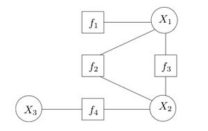
Consider a function that factorizes as follows:

[math]\displaystyle{ g(X_1,X_2,X_3) = f_1(X_1)f_2(X_1,X_2)f_3(X_1,X_2)f_4(X_2,X_3) }[/math],

with a corresponding factor graph shown on the right. Observe that the factor graph has a cycle. If we merge [math]\displaystyle{ f_2(X_1,X_2)f_3(X_1,X_2) }[/math] into a single factor, the resulting factor graph will be a tree. This is an important distinction, as message passing algorithms are usually exact for trees, but only approximate for graphs with cycles.

Message passing on factor graphs

A popular message passing algorithm on factor graphs is the sum–product algorithm, which efficiently computes all the marginals of the individual variables of the function. In particular, the marginal of variable [math]\displaystyle{ X_k }[/math] is defined as

[math]\displaystyle{ g_k(X_k) = \sum_{X_{\bar{k}}} g(X_1,X_2,\dots,X_n) }[/math]

where the notation [math]\displaystyle{ X_{\bar{k}} }[/math] means that the summation goes over all the variables, except [math]\displaystyle{ X_k }[/math]. The messages of the sum–product algorithm are conceptually computed in the vertices and passed along the edges. A message from or to a variable vertex is always a function of that particular variable. For instance, when a variable is binary, the messages over the edges incident to the corresponding vertex can be represented as vectors of length 2: the first entry is the message evaluated in 0, the second entry is the message evaluated in 1. When a variable belongs to the field of real numbers, messages can be arbitrary functions, and special care needs to be taken in their representation.

In practice, the sum–product algorithm is used for statistical inference, whereby [math]\displaystyle{ g(X_1,X_2,\dots,X_n) }[/math] is a joint distribution or a joint likelihood function, and the factorization depends on the conditional independencies among the variables.

The Hammersley–Clifford theorem shows that other probabilistic models such as Bayesian networks and Markov networks can be represented as factor graphs; the latter representation is frequently used when performing inference over such networks using belief propagation. On the other hand, Bayesian networks are more naturally suited for generative models, as they can directly represent the causalities of the model.

See also

• Belief propagation
• Bayesian inference
• Bayesian programming
• Conditional probability
• Markov network
• Bayesian network
• Hammersley–Clifford theorem

External links

• Loeliger, Hans-Andrea (January 2004), "An Introduction to Factor Graphs"], IEEE Signal Processing Magazine 21 (1): 28–41, doi:10.1109/MSP.2004.1267047, Bibcode: 2004ISPM...21...28L, http://www.isiweb.ee.ethz.ch/papers/arch/aloe-2004-spmagffg.pdf 
• dimple an open-source tool for building and solving factor graphs in MATLAB.
• Loeliger, Hans-Andrea (2008), An introduction to Factor Graphs, http://people.binf.ku.dk/~thamelry/MLSB08/hal.pdf 

References

• Clifford (1990), "Markov random fields in statistics", in Grimmett, G.R.; Welsh, D.J.A. (postscript), Disorder in Physical Systems, J.M. Hammersley Festschrift, Oxford University Press, pp. 19–32, ISBN 9780198532156, http://www.statslab.cam.ac.uk/~grg/books/hammfest/3-pdc.ps 
• Frey, Brendan J. (2003), "Extending Factor Graphs so as to Unify Directed and Undirected Graphical Models", in Jain, Nitin, UAI'03, Proceedings of the 19th Conference in Uncertainty in Artificial Intelligence, Morgan Kaufmann, pp. 257–264, ISBN 0127056645, https://dl.acm.org/doi/abs/10.5555/2100584.2100615 
• Kschischang, Frank R.; Frey, Brendan J.; Loeliger, Hans-Andrea (2001), "Factor Graphs and the Sum-Product Algorithm", IEEE Transactions on Information Theory 47 (2): 498–519, doi:10.1109/18.910572. 
• Wymeersch, Henk (2007), Iterative Receiver Design, Cambridge University Press, ISBN 978-0-521-87315-4, http://www.cambridge.org/us/catalogue/catalogue.asp?isbn=9780521873154