Inverse-gamma distribution

Short description: Two-parameter family of continuous probability distributions

Inverse-gamma

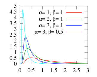
Probability density function
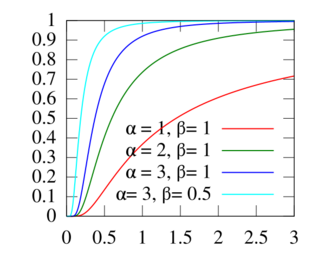
Cumulative distribution function
Parameters	[math]\displaystyle{ \alpha\gt 0 }[/math] shape (real) [math]\displaystyle{ \beta\gt 0 }[/math] scale (real)
Support	[math]\displaystyle{ x\in(0,\infty)\! }[/math]
PDF	[math]\displaystyle{ \frac{\beta^\alpha}{\Gamma(\alpha)} x^{-\alpha - 1} \exp \left(-\frac{\beta}{x}\right) }[/math]
CDF	[math]\displaystyle{ \frac{\Gamma(\alpha,\beta/x)}{\Gamma(\alpha)} \! }[/math]
Mean	[math]\displaystyle{ \frac{\beta }{\alpha-1}\! }[/math] for [math]\displaystyle{ \alpha \gt 1 }[/math]
Mode	[math]\displaystyle{ \frac{\beta}{\alpha+1}\! }[/math]
Variance	[math]\displaystyle{ \frac{\beta^2}{(\alpha-1)^2(\alpha-2)}\! }[/math] for [math]\displaystyle{ \alpha \gt 2 }[/math]
Skewness	[math]\displaystyle{ \frac{4\sqrt{\alpha-2}}{\alpha-3}\! }[/math] for [math]\displaystyle{ \alpha \gt 3 }[/math]
Kurtosis	[math]\displaystyle{ \frac{6(5\,\alpha-11)}{(\alpha-3)(\alpha-4)}\! }[/math] for [math]\displaystyle{ \alpha \gt 4 }[/math]
Entropy	[math]\displaystyle{ \alpha\!+\!\ln(\beta\Gamma(\alpha))\!-\!(1\!+\!\alpha)\psi(\alpha) }[/math] (see digamma function)
MGF	Does not exist.
CF	[math]\displaystyle{ \frac{2\left(-i\beta t\right)^{\!\!\frac{\alpha}{2}}}{\Gamma(\alpha)}K_{\alpha}\left(\sqrt{-4i\beta t}\right) }[/math]

In probability theory and statistics, the inverse gamma distribution is a two-parameter family of continuous probability distributions on the positive real line, which is the distribution of the reciprocal of a variable distributed according to the gamma distribution.

Perhaps the chief use of the inverse gamma distribution is in Bayesian statistics, where the distribution arises as the marginal posterior distribution for the unknown variance of a normal distribution, if an uninformative prior is used, and as an analytically tractable conjugate prior, if an informative prior is required. It is common among some Bayesians to consider an alternative parametrization of the normal distribution in terms of the precision, defined as the reciprocal of the variance, which allows the gamma distribution to be used directly as a conjugate prior. Other Bayesians prefer to parametrize the inverse gamma distribution differently, as a scaled inverse chi-squared distribution.

Characterization

Probability density function

The inverse gamma distribution's probability density function is defined over the support [math]\displaystyle{ x \gt 0 }[/math]

[math]\displaystyle{ f(x; \alpha, \beta) = \frac{\beta^\alpha}{\Gamma(\alpha)} (1/x)^{\alpha + 1}\exp\left(-\beta/x\right) }[/math]

with shape parameter [math]\displaystyle{ \alpha }[/math] and scale parameter [math]\displaystyle{ \beta }[/math]. Here [math]\displaystyle{ \Gamma(\cdot) }[/math] denotes the gamma function.

Unlike the Gamma distribution, which contains a somewhat similar exponential term, [math]\displaystyle{ \beta }[/math] is a scale parameter as the distribution function satisfies:

[math]\displaystyle{ f(x; \alpha, \beta) = \frac{f(x / \beta; \alpha, 1)}{\beta} }[/math]

Cumulative distribution function

The cumulative distribution function is the regularized gamma function

[math]\displaystyle{ F(x; \alpha, \beta) = \frac{\Gamma\left(\alpha,\frac{\beta}{x}\right)}{\Gamma(\alpha)} = Q\left(\alpha, \frac{\beta}{x}\right)\! }[/math]

where the numerator is the upper incomplete gamma function and the denominator is the gamma function. Many math packages allow direct computation of [math]\displaystyle{ Q }[/math], the regularized gamma function.

Moments

Provided that [math]\displaystyle{ \alpha \gt n }[/math], the [math]\displaystyle{ n }[/math]-th moment of the inverse gamma distribution is given by

[math]\displaystyle{ \mathrm{E}[X^n] = \beta^n \frac{\Gamma(\alpha - n)}{\Gamma(\alpha)} = \frac{\beta^n}{(\alpha - 1) \cdots (\alpha - n)}. }[/math]

Characteristic function

[math]\displaystyle{ K_{\alpha}(\cdot) }[/math] in the expression of the characteristic function is the modified Bessel function of the 2nd kind.

Properties

For [math]\displaystyle{ \alpha\gt 0 }[/math] and [math]\displaystyle{ \beta\gt 0 }[/math],

[math]\displaystyle{ \mathbb{E}[\ln(X)] = \ln(\beta) - \psi(\alpha)\, }[/math]

and

[math]\displaystyle{ \mathbb{E}[X^{-1}] = \frac{\alpha}{\beta},\, }[/math]

The information entropy is

[math]\displaystyle{ \begin{align} \operatorname{H}(X) & = \operatorname{E}[-\ln(p(X))] \\ & = \operatorname{E}\left[-\alpha \ln(\beta) + \ln(\Gamma(\alpha)) + (\alpha+1)\ln(X) + \frac{\beta}{X}\right] \\ & = -\alpha \ln(\beta) + \ln(\Gamma(\alpha)) + (\alpha+1)\ln(\beta) - (\alpha+1)\psi(\alpha) + \alpha\\ & = \alpha + \ln(\beta\Gamma(\alpha)) - (\alpha+1)\psi(\alpha). \end{align} }[/math]

where [math]\displaystyle{ \psi(\alpha) }[/math] is the digamma function.

The Kullback-Leibler divergence of Inverse-Gamma(α_p, β_p) from Inverse-Gamma(α_q, β_q) is the same as the KL-divergence of Gamma(α_p, β_p) from Gamma(α_q, β_q):

[math]\displaystyle{ D_{\mathrm{KL}}(\alpha_p,\beta_p; \alpha_q, \beta_q) = \mathbb{E}\left[ \log \frac{\rho(X)}{\pi(X)}\right] = \mathbb{E}\left[ \log \frac{\rho(1/Y)}{\pi(1/Y)}\right] = \mathbb{E}\left[ \log \frac{\rho_G(Y)}{\pi_G(Y)}\right], }[/math]

where [math]\displaystyle{ \rho, \pi }[/math] are the pdfs of the Inverse-Gamma distributions and [math]\displaystyle{ \rho_G, \pi_G }[/math] are the pdfs of the Gamma distributions, [math]\displaystyle{ Y }[/math] is Gamma(α_p, β_p) distributed.

[math]\displaystyle{ \begin{align} D_{\mathrm{KL}}(\alpha_p,\beta_p; \alpha_q, \beta_q) = {} & (\alpha_p-\alpha_q) \psi(\alpha_p) - \log\Gamma(\alpha_p) + \log\Gamma(\alpha_q) + \alpha_q(\log \beta_p - \log \beta_q) + \alpha_p\frac{\beta_q-\beta_p}{\beta_p}. \end{align} }[/math]

Related distributions

• If [math]\displaystyle{ X \sim \mbox{Inv-Gamma}(\alpha, \beta) }[/math] then [math]\displaystyle{ k X \sim \mbox{Inv-Gamma}(\alpha, k \beta) \, }[/math], for [math]\displaystyle{ k \gt 0 }[/math]
• If [math]\displaystyle{ X \sim \mbox{Inv-Gamma}(\alpha, \tfrac{1}{2}) }[/math] then [math]\displaystyle{ X \sim \mbox{Inv-}\chi^2(2 \alpha)\, }[/math] (inverse-chi-squared distribution)
• If [math]\displaystyle{ X \sim \mbox{Inv-Gamma}(\tfrac{\alpha}{2}, \tfrac{1}{2}) }[/math] then [math]\displaystyle{ X \sim \mbox{Scaled Inv-}\chi^2(\alpha,\tfrac{1}{\alpha})\, }[/math] (scaled-inverse-chi-squared distribution)
• If [math]\displaystyle{ X \sim \textrm{Inv-Gamma}(\tfrac{1}{2},\tfrac{c}{2}) }[/math] then [math]\displaystyle{ X \sim \textrm{Levy}(0,c)\, }[/math] (Lévy distribution)
• If [math]\displaystyle{ X \sim \textrm{Inv-Gamma}(1,c) }[/math] then [math]\displaystyle{ \tfrac{1}{X} \sim \textrm{Exp}(c)\, }[/math] (Exponential distribution)
• If [math]\displaystyle{ X \sim \mbox{Gamma}(\alpha, \beta)\, }[/math] (Gamma distribution with rate parameter [math]\displaystyle{ \beta }[/math]) then [math]\displaystyle{ \tfrac{1}{X} \sim \mbox{Inv-Gamma}(\alpha, \beta)\, }[/math] (see derivation in the next paragraph for details)
• Note that If [math]\displaystyle{ X \sim \mbox{Gamma}(k, \theta) }[/math] (Gamma distribution with scale parameter [math]\displaystyle{ \theta }[/math] ) then [math]\displaystyle{ 1/X \sim \mbox{Inv-Gamma}(k, 1/\theta) }[/math]
• Inverse gamma distribution is a special case of type 5 Pearson distribution
• A multivariate generalization of the inverse-gamma distribution is the inverse-Wishart distribution.
• For the distribution of a sum of independent inverted Gamma variables see Witkovsky (2001)

Derivation from Gamma distribution

Let [math]\displaystyle{ X \sim \mbox{Gamma}(\alpha, \beta) }[/math], and recall that the pdf of the gamma distribution is

[math]\displaystyle{ f_{X}(x) = \frac{\beta^\alpha}{\Gamma(\alpha)}x^{\alpha-1}e^{-\beta x} }[/math], [math]\displaystyle{ x \gt 0 }[/math].

Note that [math]\displaystyle{ \beta }[/math] is the rate parameter from the perspective of the gamma distribution.

Define the transformation [math]\displaystyle{ Y = g(X) = \tfrac{1}{X} }[/math]. Then, the pdf of [math]\displaystyle{ Y }[/math] is

[math]\displaystyle{ \begin{align} f_Y(y) &= f_X \left( g^{-1}(y) \right) \left| \frac{d}{dy} g^{-1}(y) \right| \\[6pt] &= \frac{\beta^\alpha}{\Gamma(\alpha)} \left( \frac{1}{y} \right)^{\alpha-1} \exp \left( \frac{-\beta}{y} \right) \frac{1}{y^2} \\[6pt] &= \frac{\beta^\alpha}{\Gamma(\alpha)} \left( \frac{1}{y} \right)^{\alpha+1} \exp \left( \frac{-\beta}{y} \right) \\[6pt] &= \frac{\beta^\alpha}{\Gamma(\alpha)} \left( y \right)^{-\alpha-1} \exp \left( \frac{-\beta}{y} \right) \\[6pt] \end{align} }[/math]

Note that [math]\displaystyle{ \beta }[/math] is the scale parameter from the perspective of the inverse gamma distribution. This can be straightforwardly demonstrated by seeing that [math]\displaystyle{ \beta }[/math] satisfies the conditions for being a scale parameter.

[math]\displaystyle{ \begin{align} \frac{f_{\beta}(y / \beta)}{\beta} &= \frac{1}{\beta} \frac{\beta^\alpha}{\Gamma(\alpha)} \left( \frac{y}{\beta} \right)^{-\alpha-1} \exp(-y) \\[6pt] &= \frac{1}{\Gamma(\alpha)} \left( y \right)^{-\alpha-1} \exp(-y) \\[6pt] &= f_{\beta=1}(y) \end{align} }[/math]

Occurrence

• Hitting time distribution of a Wiener process follows a Lévy distribution, which is a special case of the inverse-gamma distribution with [math]\displaystyle{ \alpha=0.5 }[/math].

See also

• Gamma distribution
• Inverse-chi-squared distribution
• Normal distribution
• Pearson distribution

References

• Hoff, P. (2009). "A first course in bayesian statistical methods". Springer.
• Witkovsky, V. (2001). "Computing the Distribution of a Linear Combination of Inverted Gamma Variables". Kybernetika 37 (1): 79–90.