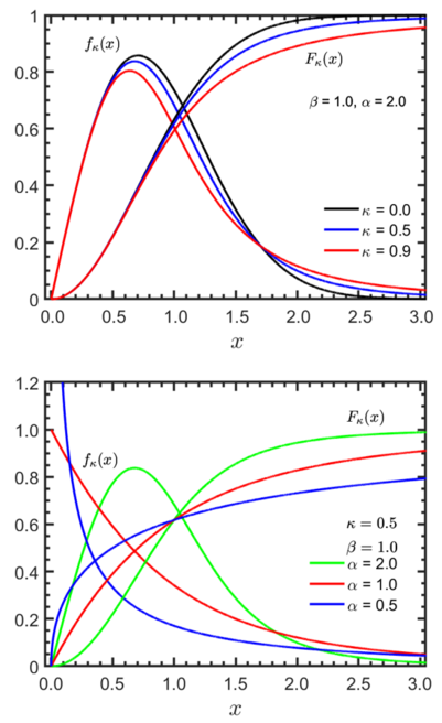
Kaniadakis Weibull distribution

Short description: Continuous probability distribution

κ-Weibull distribution

Probability density function
Cumulative distribution function
Parameters	[math]\displaystyle{ 0 \lt \kappa \lt 1 }[/math] [math]\displaystyle{ \alpha \gt 0 }[/math] rate shape (real) [math]\displaystyle{ \beta\gt 0 }[/math] rate (real)
Support	[math]\displaystyle{ x \in [0, +\infty) }[/math]
PDF	[math]\displaystyle{ \frac{ \alpha \beta x^{ \alpha - 1 } } { \sqrt{ 1 + \kappa^2 \beta^2 x^{2 \alpha} } } \exp_\kappa ( - \beta x^\alpha ) }[/math]
CDF	[math]\displaystyle{ 1 - \exp_\kappa(-\beta x^\alpha) }[/math]
Quantile	[math]\displaystyle{ \beta^{-1 / \alpha } \Bigg[ \ln_\kappa \Bigg(\frac{1}{1 - F_\kappa} \Bigg) \Bigg]^{1/ \alpha} }[/math]
Median	[math]\displaystyle{ \beta^{-1/\alpha} \Bigg(\ln_\kappa (2)\Bigg)^{1/\alpha} }[/math]
Mode	[math]\displaystyle{ \beta^{ -1 / \alpha } \Bigg( \frac{ \alpha^2 + 2 \kappa^2 (\alpha - 1 )}{ 2 \kappa^2 ( \alpha^2 - \kappa^2)} \sqrt{1 + \frac{4 \kappa^2 (\alpha^2 - \kappa^2 )( \alpha - 1)^2}{ [ \alpha^2 + 2 \kappa^2 (\alpha - 1) ]^2} } - 1 \Bigg)^{1/2 \alpha} }[/math]

The Kaniadakis Weibull distribution (or κ-Weibull distribution) is a probability distribution arising as a generalization of the Weibull distribution. It is one example of a Kaniadakis κ-distribution. The κ-Weibull distribution has been adopted successfully for describing a wide variety of complex systems in seismology, economy, epidemiology, among many others.

Definitions

Probability density function

The Kaniadakis κ-Weibull distribution is exhibits power-law right tails, and it has the following probability density function:

[math]\displaystyle{ f_{_{\kappa}}(x) = \frac{\alpha \beta x^{\alpha-1}}{\sqrt{1+\kappa^2 \beta^2 x^{2\alpha} }} \exp_\kappa(-\beta x^\alpha) }[/math]

valid for [math]\displaystyle{ x \geq 0 }[/math], where [math]\displaystyle{ |\kappa| \lt 1 }[/math] is the entropic index associated with the Kaniadakis entropy, [math]\displaystyle{ \beta \gt 0 }[/math] is the scale parameter, and [math]\displaystyle{ \alpha \gt 0 }[/math] is the shape parameter or Weibull modulus.

The Weibull distribution is recovered as [math]\displaystyle{ \kappa \rightarrow 0. }[/math]

Cumulative distribution function

The cumulative distribution function of κ-Weibull distribution is given by

[math]\displaystyle{ F_\kappa(x) = 1 - \exp_\kappa(-\beta x^\alpha) }[/math]

valid for [math]\displaystyle{ x \geq 0 }[/math]. The cumulative Weibull distribution is recovered in the classical limit [math]\displaystyle{ \kappa \rightarrow 0 }[/math].

Survival distribution and hazard functions

The survival distribution function of κ-Weibull distribution is given by

[math]\displaystyle{ S_\kappa(x) = \exp_\kappa(-\beta x^\alpha) }[/math]

valid for [math]\displaystyle{ x \geq 0 }[/math]. The survival Weibull distribution is recovered in the classical limit [math]\displaystyle{ \kappa \rightarrow 0 }[/math].

Comparison between the Kaniadakis κ-Weibull probability function and its cumulative.

The hazard function of the κ-Weibull distribution is obtained through the solution of the κ-rate equation:

[math]\displaystyle{ \frac{ S_\kappa(x) }{ dx } = -h_\kappa S_\kappa(x) }[/math]

with [math]\displaystyle{ S_\kappa(0) = 1 }[/math], where [math]\displaystyle{ h_\kappa }[/math] is the hazard function:

[math]\displaystyle{ h_\kappa = \frac{\alpha \beta x^{\alpha-1}}{\sqrt{1+\kappa^2 \beta^2 x^{2\alpha} }} }[/math]

The cumulative κ-Weibull distribution is related to the κ-hazard function by the following expression:

[math]\displaystyle{ S_\kappa = e^{-H_\kappa(x)} }[/math]

where

[math]\displaystyle{ H_\kappa (x) = \int_0^x h_\kappa(z) dz }[/math]

[math]\displaystyle{ H_\kappa (x) = \frac{1}{\kappa} \textrm{arcsinh}\left(\kappa \beta x^\alpha \right) }[/math]

is the cumulative κ-hazard function. The cumulative hazard function of the Weibull distribution is recovered in the classical limit [math]\displaystyle{ \kappa \rightarrow 0 }[/math]: [math]\displaystyle{ H(x) = \beta x^\alpha }[/math] .

Properties

Moments, median and mode

The κ-Weibull distribution has moment of order [math]\displaystyle{ m \in \mathbb{N} }[/math] given by

[math]\displaystyle{ \operatorname{E}[X^m] = \frac{|2\kappa \beta|^{-m/\alpha}}{1+\kappa \frac{m}{\alpha}} \frac{\Gamma\Big(\frac{1}{2\kappa}-\frac{m}{2\alpha}\Big)}{\Gamma\Big(\frac{1}{2\kappa}+\frac{m}{2\alpha}\Big)} \Gamma\Big(1+\frac{m}{\alpha}\Big) }[/math]

The median and the mode are:

[math]\displaystyle{ x_{\textrm{median}} (F_\kappa) = \beta^{-1/\alpha} \Bigg(\ln_\kappa (2)\Bigg)^{1/\alpha} }[/math]

[math]\displaystyle{ x_{\textrm{mode}} = \beta^{ -1 / \alpha } \Bigg( \frac{ \alpha^2 + 2 \kappa^2 (\alpha - 1 )}{ 2 \kappa^2 ( \alpha^2 - \kappa^2)}\Bigg)^{1/2 \alpha} \Bigg( \sqrt{1 + \frac{4 \kappa^2 (\alpha^2 - \kappa^2 )( \alpha - 1)^2}{ [ \alpha^2 + 2 \kappa^2 (\alpha - 1) ]^2} } - 1 \Bigg)^{1/2 \alpha} \quad (\alpha \gt 1) }[/math]

Quantiles

The quantiles are given by the following expression

[math]\displaystyle{ x_{\textrm{quantile}} (F_\kappa) = \beta^{-1 / \alpha } \Bigg[ \ln_\kappa \Bigg(\frac{1}{1 - F_\kappa} \Bigg) \Bigg]^{1/ \alpha} }[/math]

with [math]\displaystyle{ 0 \leq F_\kappa \leq 1 }[/math].

Gini coefficient

The Gini coefficient is:

[math]\displaystyle{ \operatorname{G}_\kappa = 1 - \frac{\alpha + \kappa}{ \alpha + \frac{1}{2}\kappa } \frac{\Gamma\Big( \frac{1}{\kappa} - \frac{1}{2 \alpha}\Big)}{\Gamma\Big( \frac{1}{\kappa} + \frac{1}{2 \alpha}\Big)} \frac{\Gamma\Big( \frac{1}{2 \kappa} + \frac{1}{2 \alpha}\Big)}{\Gamma\Big( \frac{1}{ 2\kappa} - \frac{1}{2 \alpha}\Big)} }[/math]

Asymptotic behavior

The κ-Weibull distribution II behaves asymptotically as follows:

[math]\displaystyle{ \lim_{x \to +\infty} f_\kappa (x) \sim \frac{\alpha}{\kappa} (2 \kappa \beta)^{-1/\kappa} x^{-1 - \alpha/\kappa} }[/math]

[math]\displaystyle{ \lim_{x \to 0^+} f_\kappa (x) = \alpha \beta x^{\alpha - 1} }[/math]

Related distributions

• The κ-Weibull distribution is a generalization of:
  • κ-Exponential distribution of type II, when [math]\displaystyle{ \alpha = 1 }[/math];
  • Exponential distribution when [math]\displaystyle{ \kappa = 0 }[/math] and [math]\displaystyle{ \alpha = 1 }[/math].
• A κ-Weibull distribution corresponds to a κ-deformed Rayleigh distribution when [math]\displaystyle{ \alpha = 2 }[/math] and a Rayleigh distribution when [math]\displaystyle{ \kappa = 0 }[/math] and [math]\displaystyle{ \alpha = 2 }[/math].

Applications

The κ-Weibull distribution has been applied in several areas, such as:

• In economy, for analyzing personal income models, in order to accurately describing simultaneously the income distribution among the richest part and the great majority of the population.
• In seismology, the κ-Weibull represents the statistical distribution of magnitude of the earthquakes distributed across the Earth, generalizing the Gutenberg–Richter law, and the interval distributions of seismic data, modeling extreme-event return intervals.
• In epidemiology, the κ-Weibull distribution presents a universal feature for epidemiological analysis.

See also

• Giorgio Kaniadakis
• Kaniadakis statistics
• Kaniadakis distribution
• Kaniadakis κ-Exponential distribution
• Kaniadakis κ-Gaussian distribution
• Kaniadakis κ-Gamma distribution
• Kaniadakis κ-Logistic distribution
• Kaniadakis κ-Erlang distribution

External links

• Kaniadakis Statistics on arXiv.org

References

- ↑ 1.0 1.1 Clementi, F.; Gallegati, M.; Kaniadakis, G. (2007). "κ-generalized statistics in personal income distribution" (in en). The European Physical Journal B 57 (2): 187–193. doi:10.1140/epjb/e2007-00120-9. ISSN 1434-6028. Bibcode: 2007EPJB...57..187C. http://link.springer.com/10.1140/epjb/e2007-00120-9.
- ↑ Clementi, F.; Di Matteo, T.; Gallegati, M.; Kaniadakis, G. (2008). "The -generalized distribution: A new descriptive model for the size distribution of incomes" (in en). Physica A: Statistical Mechanics and Its Applications 387 (13): 3201–3208. doi:10.1016/j.physa.2008.01.109. https://linkinghub.elsevier.com/retrieve/pii/S0378437108001349.
- ↑ 3.0 3.1 3.2 Kaniadakis, G. (2021-01-01). "New power-law tailed distributions emerging in κ-statistics (a)". Europhysics Letters 133 (1): 10002. doi:10.1209/0295-5075/133/10002. ISSN 0295-5075. Bibcode: 2021EL....13310002K. https://iopscience.iop.org/article/10.1209/0295-5075/133/10002.
- ↑ Clementi, Fabio; Gallegati, Mauro; Kaniadakis, Giorgio (October 2010). "A model of personal income distribution with application to Italian data" (in en). Empirical Economics 39 (2): 559–591. doi:10.1007/s00181-009-0318-2. ISSN 0377-7332. http://link.springer.com/10.1007/s00181-009-0318-2.
- ↑ Clementi, F; Gallegati, M; Kaniadakis, G (2012-12-06). "A generalized statistical model for the size distribution of wealth". Journal of Statistical Mechanics: Theory and Experiment 2012 (12): P12006. doi:10.1088/1742-5468/2012/12/P12006. ISSN 1742-5468. Bibcode: 2012JSMTE..12..006C. https://iopscience.iop.org/article/10.1088/1742-5468/2012/12/P12006.
- ↑ da Silva, Sérgio Luiz E.F. (2021). "κ -generalised Gutenberg–Richter law and the self-similarity of earthquakes" (in en). Chaos, Solitons & Fractals 143: 110622. doi:10.1016/j.chaos.2020.110622. Bibcode: 2021CSF...14310622D. https://linkinghub.elsevier.com/retrieve/pii/S0960077920310134.
- ↑ Hristopulos, Dionissios T.; Petrakis, Manolis P.; Kaniadakis, Giorgio (2014-05-28). "Finite-size effects on return interval distributions for weakest-link-scaling systems" (in en). Physical Review E 89 (5): 052142. doi:10.1103/PhysRevE.89.052142. ISSN 1539-3755. PMID 25353774. Bibcode: 2014PhRvE..89e2142H. https://link.aps.org/doi/10.1103/PhysRevE.89.052142.
- ↑ Hristopulos, Dionissios; Petrakis, Manolis; Kaniadakis, Giorgio (2015-03-09). "Weakest-Link Scaling and Extreme Events in Finite-Sized Systems" (in en). Entropy 17 (3): 1103–1122. doi:10.3390/e17031103. ISSN 1099-4300. Bibcode: 2015Entrp..17.1103H.
- ↑ Kaniadakis, Giorgio; Baldi, Mauro M.; Deisboeck, Thomas S.; Grisolia, Giulia; Hristopulos, Dionissios T.; Scarfone, Antonio M.; Sparavigna, Amelia; Wada, Tatsuaki et al. (2020). "The κ-statistics approach to epidemiology" (in en). Scientific Reports 10 (1): 19949. doi:10.1038/s41598-020-76673-3. ISSN 2045-2322. PMID 33203913. Bibcode: 2020NatSR..1019949K.