Rayleigh distribution

Short description: Probability distribution

Rayleigh

Probability density function
Cumulative distribution function
Parameters	scale: $\sigma >0$
Support	$x\in [0,\mathrm{\infty })$
PDF	$\frac{x}{{\sigma }^2}{e}^{-x^2/\left(2{\sigma }^2\right)}$
CDF	$1-e^{-x^2/\left(2{\sigma }^2\right)}$
Quantile	$Q(F;\sigma )=\sigma \sqrt{-2\ln (1-F)}$
Mean	$\sigma \sqrt{\frac{\pi }{2}}$
Median	$\sigma \sqrt{2\ln (2)}$
Mode	$\sigma$
Variance	$\frac{4-\pi }{2}{\sigma }^2$
Skewness	$\frac{2\sqrt{\pi }(\pi -3)}{(4-\pi {)}^{3/2}}$
Kurtosis	$-\frac{6{\pi }^2-24\pi +16}{(4-\pi {)}^2}$
Entropy	$1+\ln \left(\frac{\sigma }{\sqrt{2}}\right)+\frac{\gamma }{2}$
MGF	$1+\sigma t{e}^{{\sigma }^2{t}^2/2}\sqrt{\frac{\pi }{2}}(\mathrm{erf}\left(\frac{\sigma t}{\sqrt{2}}\right)+1)$
CF	$1-\sigma t{e}^{-{\sigma }^2{t}^2/2}\sqrt{\frac{\pi }{2}}(\mathrm{erfi}\left(\frac{\sigma t}{\sqrt{2}}\right)-i)$

In probability theory and statistics, the Rayleigh distribution is a continuous probability distribution for nonnegative-valued random variables. Up to rescaling, it coincides with the chi distribution with two degrees of freedom. The distribution is named after Lord Rayleigh (/ˈreɪli/).

A Rayleigh distribution is often observed when the overall magnitude of a vector in the plane is related to its directional components. One example where the Rayleigh distribution naturally arises is when wind velocity is analyzed in two dimensions. Assuming that each component is uncorrelated, normally distributed with equal variance, and zero mean, then the overall wind speed (vector magnitude) will be characterized by a Rayleigh distribution. A second example of the distribution arises in the case of random complex numbers whose real and imaginary components are independently and identically distributed Gaussian with equal variance and zero mean. In that case, the absolute value of the complex number is Rayleigh-distributed.

Definition

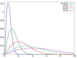
The probability density function of the Rayleigh distribution is

$f(x;\sigma )=\frac{x}{{\sigma }^2}{e}^{-x^2/(2{\sigma }^2)},x\ge 0,$

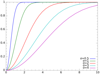
where $\sigma$ is the scale parameter of the distribution. The cumulative distribution function is

$F(x;\sigma )=1-e^{-x^2/(2{\sigma }^2)}$

for $x\in [0,\mathrm{\infty }).$

Relation to random vector length

Consider the two-dimensional vector $Y=(U,V)$ which has components that are bivariate normally distributed, centered at zero, and independent. Then $U$ and $V$ have density functions

$f_U(x;\sigma )=f_V(x;\sigma )=\frac{e^{-x^2/(2{\sigma }^2)}}{\sqrt{2\pi {\sigma }^2}}.$

Let $X$ be the length of $Y$. That is, $X=\sqrt{U^2+V^2}.$ Then $X$ has cumulative distribution function

$F_X(x;\sigma )=\underset{D_x}{\iint }{f}_U(u;\sigma )f_V(v;\sigma )dA,$

where $D_x$ is the disk

$D_x=\{(u,v):\sqrt{u^2+v^2}\le x\}.$

Writing the double integral in polar coordinates, it becomes

$F_X(x;\sigma )=\frac{1}{2\pi {\sigma }^2}\underset{0}{\overset{2\pi }{\int }}\underset{0}{\overset{x}{\int }}r{e}^{-r^2/(2{\sigma }^2)}drd\theta =\frac{1}{{\sigma }^2}\underset{0}{\overset{x}{\int }}r{e}^{-r^2/(2{\sigma }^2)}dr.$

Finally, the probability density function for $X$ is the derivative of its cumulative distribution function, which by the fundamental theorem of calculus is

$f_X(x;\sigma )=\frac{d}{dx}{F}_X(x;\sigma )=\frac{x}{{\sigma }^2}{e}^{-x^2/(2{\sigma }^2)},$

which is the Rayleigh distribution. It is straightforward to generalize to vectors of dimension other than 2. There are also generalizations when the components have unequal variance or correlations (Hoyt distribution), or when the vector Y follows a bivariate Student t-distribution (see also: Hotelling's T-squared distribution).

Generalization to bivariate Student's t-distribution

Suppose $Y$ is a random vector with components $u,v$ that follows a multivariate t-distribution. If the components both have mean zero, equal variance, and are independent, the bivariate Student's-t distribution takes the form: $f(u,v)=\frac{1}{2\pi {\sigma }^2}{(1+\frac{u^2+v^2}{\nu {\sigma }^2})}^{-\nu /2-1}$ Let $R=\sqrt{U^2+V^2}$ be the magnitude of $Y$. Then the cumulative distribution function (CDF) of the magnitude is: $F(r)=\frac{1}{2\pi {\sigma }^2}\underset{D_r}{\iint }{(1+\frac{u^2+v^2}{\nu {\sigma }^2})}^{-\nu /2-1}dudv$ where $D_r$ is the disk defined by: $D_r=\{(u,v):\sqrt{u^2+v^2}\le r\}$ Converting to polar coordinates leads to the CDF becoming: $\begin{array}{rl}F(r)& =\frac{1}{2\pi {\sigma }^2}\underset{0}{\overset{r}{\int }}\underset{0}{\overset{2\pi }{\int }}\rho {(1+\frac{{\rho }^2}{\nu {\sigma }^2})}^{-\nu /2-1}d\theta d\rho \\ & =\frac{1}{{\sigma }^2}\underset{0}{\overset{r}{\int }}\rho {(1+\frac{{\rho }^2}{\nu {\sigma }^2})}^{-\nu /2-1}d\rho \\ & =1-{(1+\frac{r^2}{\nu {\sigma }^2})}^{-\nu /2}\end{array}$ Finally, the probability density function (PDF) of the magnitude may be derived: $f(r)=F^{\prime }(r)=\frac{r}{{\sigma }^2}{(1+\frac{r^2}{\nu {\sigma }^2})}^{-\nu /2-1}$ In the limit as $\nu \to \mathrm{\infty }$, the Rayleigh distribution is recovered because: $\underset{\nu \to \mathrm{\infty }}{\lim }{(1+\frac{r^2}{\nu {\sigma }^2})}^{-\nu /2-1}=e^{-r^2/2{\sigma }^2}$

Properties

The raw moments are given by:

${\mu }_j={\sigma }^j{2}^{j/2}\mathrm{\Gamma }(1+\frac{j}{2}),$

where $\mathrm{\Gamma }(z)$ is the gamma function.

The mean of a Rayleigh random variable is thus :

$\mu (X)=\sigma \sqrt{\frac{\pi }{2}}\approx 1.253\sigma .$

The standard deviation of a Rayleigh random variable is:

$\mathrm{std}(X)=\sqrt{(2-\frac{\pi }{2})}\sigma \approx 0.655\sigma$

The variance of a Rayleigh random variable is :

$\mathrm{var}(X)={\mu }_2-{\mu }_1^2=(2-\frac{\pi }{2}){\sigma }^2\approx 0.429{\sigma }^2$

The mode is $\sigma ,$ and the maximum pdf is

$f_{\max }=f(\sigma ;\sigma )=\frac{1}{\sigma }{e}^{-1/2}\approx \frac{0.606}{\sigma }.$

The skewness is given by:

${\gamma }_1=\frac{2\sqrt{\pi }(\pi -3)}{(4-\pi {)}^{3/2}}\approx 0.631$

The excess kurtosis is given by:

${\gamma }_2=-\frac{6{\pi }^2-24\pi +16}{(4-\pi {)}^2}\approx 0.245$

The characteristic function is given by:

$\phi (t)=1-\sigma t{e}^{-\frac{1}{2}{\sigma }^2{t}^2}\sqrt{\frac{\pi }{2}}[\mathrm{erfi}\left(\frac{\sigma t}{\sqrt{2}}\right)-i]$

where $\mathrm{erfi}(z)$ is the imaginary error function. The moment generating function is given by

$M(t)=1+\sigma t{e}^{\frac{1}{2}{\sigma }^2{t}^2}\sqrt{\frac{\pi }{2}}[\mathrm{erf}\left(\frac{\sigma t}{\sqrt{2}}\right)+1]$

where $\mathrm{erf}(z)$ is the error function.

Differential entropy

The differential entropy is given by

$H=1+\ln \left(\frac{\sigma }{\sqrt{2}}\right)+\frac{\gamma }{2}$

where $\gamma$ is the Euler–Mascheroni constant.

Parameter estimation

Given a sample of N independent and identically distributed Rayleigh random variables $x_i$ with parameter $\sigma$,

$\widehat{{\sigma }^2}=\frac{1}{2N}\sum _{i=1}^N{x}_i^2$ is the maximum likelihood estimate and also is unbiased.

$\hat{\sigma }\approx \sqrt{\frac{1}{2N}\sum _{i=1}^N{x}_i^2}$ is a biased estimator that can be corrected via the formula

$\sigma =\hat{\sigma }\frac{\mathrm{\Gamma }(N)\sqrt{N}}{\mathrm{\Gamma }(N+\frac{1}{2})}=\hat{\sigma }\frac{4^{N}N!(N-1)!\sqrt{N}}{(2N)!\sqrt{\pi }}$ $=\frac{\hat{\sigma }}{c_4(2N+1)}$, where c₄ is the correction factor used to unbias estimates of standard deviation for normal random variables.

Confidence intervals

To find the (1 − α) confidence interval, first find the bounds $[a,b]$ where:

  $P({\chi }_{2N}^2\le a)=\alpha /2,P({\chi }_{2N}^2\le b)=1-\alpha /2$

then the scale parameter will fall within the bounds

  $\frac{N\overline{x^2}}{b}\le \widehat{{\sigma }^2}\le \frac{N\overline{x^2}}{a}$

Generating random variates

Given a random variate U drawn from the uniform distribution in the interval (0, 1), then the variate

$X=\sigma \sqrt{-2\ln U}$

has a Rayleigh distribution with parameter $\sigma$. This is obtained by applying the inverse transform sampling-method.

Related distributions

• $R\sim \mathrm{R}\mathrm{a}\mathrm{y}\mathrm{l}\mathrm{e}\mathrm{i}\mathrm{g}\mathrm{h}(\sigma )$ is Rayleigh distributed if $R=\sqrt{X^2+Y^2}$, where $X\sim N(0,{\sigma }^2)$ and $Y\sim N(0,{\sigma }^2)$ are independent normal random variables. This gives motivation to the use of the symbol $\sigma$ in the above parametrization of the Rayleigh density.
• The magnitude $|z|$ of a standard complex normally distributed variable z is Rayleigh distributed.
• The chi distribution with v = 2 is equivalent to the Rayleigh Distribution with σ = 1: $R(\sigma )\sim \sigma {\chi }_2^{}.$
• If $R\sim \mathrm{R}\mathrm{a}\mathrm{y}\mathrm{l}\mathrm{e}\mathrm{i}\mathrm{g}\mathrm{h}(1)$, then $R^2$ has a chi-squared distribution with 2 degrees of freedom: $[Q=R(\sigma {)}^2]\sim {\sigma }^2{\chi }_2^2.$
• If $R\sim \mathrm{R}\mathrm{a}\mathrm{y}\mathrm{l}\mathrm{e}\mathrm{i}\mathrm{g}\mathrm{h}(\sigma )$, then $\sum _{i=1}^N{R}_i^2$ has a gamma distribution with parameters $N$ and $\frac{1}{2{\sigma }^2}$

  $[Y=\sum _{i=1}^N{R}_i^2]\sim \mathrm{\Gamma }(N,\frac{1}{2{\sigma }^2}).$

• The Rice distribution is a noncentral generalization of the Rayleigh distribution: $\mathrm{R}\mathrm{a}\mathrm{y}\mathrm{l}\mathrm{e}\mathrm{i}\mathrm{g}\mathrm{h}(\sigma )=\mathrm{R}\mathrm{i}\mathrm{c}\mathrm{e}(0,\sigma )$.
• The Weibull distribution with the shape parameter k = 2 yields a Rayleigh distribution. Then the Rayleigh distribution parameter $\sigma$ is related to the Weibull scale parameter according to $\lambda =\sigma \sqrt{2}.$
• If $X$ has an exponential distribution $X\sim \mathrm{E}\mathrm{x}\mathrm{p}\mathrm{o}\mathrm{n}\mathrm{e}\mathrm{n}\mathrm{t}\mathrm{i}\mathrm{a}\mathrm{l}(\lambda )$, then $Y=\sqrt{X}\sim \mathrm{R}\mathrm{a}\mathrm{y}\mathrm{l}\mathrm{e}\mathrm{i}\mathrm{g}\mathrm{h}(1/\sqrt{2\lambda }).$
• The half-normal distribution is the one-dimensional equivalent of the Rayleigh distribution.
• The Maxwell–Boltzmann distribution is the three-dimensional equivalent of the Rayleigh distribution.

Applications

An application of the estimation of σ can be found in magnetic resonance imaging (MRI). As MRI images are recorded as complex images but most often viewed as magnitude images, the background data is Rayleigh distributed. Hence, the above formula can be used to estimate the noise variance in an MRI image from background data.

The Rayleigh distribution was also employed in the field of nutrition for linking dietary nutrient levels and human and animal responses. In this way, the parameter σ may be used to calculate nutrient response relationship.

In the field of ballistics, the Rayleigh distribution is used for calculating the circular error probable—a measure of a gun's precision.

In physical oceanography, the distribution of significant wave height approximately follows a Rayleigh distribution.

See also

• Circular error probable
• Rayleigh fading
• Rayleigh mixture distribution
• Rice distribution

References

- ↑ "The Wave Theory of Light", Encyclopedic Britannica 1888; "The Problem of the Random Walk", Nature 1905 vol.72 p.318
- ↑ 2.0 2.1 Papoulis, Athanasios; Pillai, S. (2001) Probability, Random Variables and Stochastic Processes p. 169. ISBN 0073660116, ISBN 9780073660110
- ↑ Röver, C. (2011). "Student-t based filter for robust signal detection". Physical Review D 84 (12). doi:10.1103/physrevd.84.122004. Bibcode: 2011PhRvD..84l2004R.
- ↑ Siddiqui, M. M. (1964) "Statistical inference for Rayleigh distributions", The Journal of Research of the National Bureau of Standards, Sec. D: Radio Science, Vol. 68D, No. 9, p. 1007
- ↑ Siddiqui, M. M. (1961) "Some Problems Connected With Rayleigh Distributions", The Journal of Research of the National Bureau of Standards; Sec. D: Radio Propagation, Vol. 66D, No. 2, p. 169
- ↑ Hogema, Jeroen (2005) "Shot group statistics"
- ↑ Sijbers, J.; den Dekker, A. J.; Raman, E.; Van Dyck, D. (1999). "Parameter estimation from magnitude MR images". International Journal of Imaging Systems and Technology 10 (2): 109–114. doi:10.1002/(sici)1098-1098(1999)10:2<109::aid-ima2>3.0.co;2-r.
- ↑ den Dekker, A. J.; Sijbers, J. (2014). "Data distributions in magnetic resonance images: a review". Physica Medica 30 (7): 725–741. doi:10.1016/j.ejmp.2014.05.002. PMID 25059432.
- ↑ Ahmadi, Hamed (2017-11-21). "A mathematical function for the description of nutrient-response curve". PLOS ONE 12 (11). doi:10.1371/journal.pone.0187292. ISSN 1932-6203. PMID 29161271. Bibcode: 2017PLoSO..1287292A.
- ↑ Dean, Robert G.; Dalrymple, Robert A. (1991). Water Wave Mechanics for Engineers and Scientists. Advanced Series on Ocean Engineering - Volume 2. World Scientific. ISBN 9-789810-204211.
- ↑ "Rayleigh Probability Distribution Applied to Random Wave Heights". United States Naval Academy. https://www.usna.edu/NAOE/_files/documents/Courses/EN330/Rayleigh-Probability-Distribution-Applied-to-Random-Wave-Heights.pdf.