Lagrangian coherent structure

Short description: Distinguished surfaces of dynamic trajectories

Individual trajectories in a model flow generally show vastly different behavior from trajectories starting from the same initial condition of the real flow. This is due to the inevitable accumulation of errors and uncertainties, as well as sensitive dependence on initial conditions, in any realistic flow model. Yet an attracting LCS (such as the unstable manifold of a saddle point) is remarkably robust with respect to modelling errors and uncertainties. LCSs are, therefore, ideal tools for model validation and benchmarking

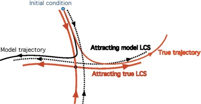
Lagrangian coherent structures (LCSs) are distinguished surfaces of trajectories in a dynamical system that exert a major influence on nearby trajectories over a time interval of interest. The type of this influence may vary, but it invariably creates a coherent trajectory pattern for which the underlying LCS serves as a theoretical centerpiece. In observations of tracer patterns in nature, one readily identifies coherent features, but it is often the underlying structure creating these features that is of interest.

As illustrated on the right, individual tracer trajectories forming coherent patterns are generally sensitive with respect to changes in their initial conditions and the system parameters. In contrast, the LCSs creating these trajectory patterns turn out to be robust and provide a simplified skeleton of the overall dynamics of the system. The robustness of this skeleton makes LCSs ideal tools for model validation, model comparison and benchmarking. LCSs can also be used for now-casting and even short-term forecasting of pattern evolution in complex dynamical systems.

Physical phenomena governed by LCSs include floating debris, oil spills, surface drifters and chlorophyll patterns in the ocean; clouds of volcanic ash and spores in the atmosphere; and coherent crowd patterns formed by humans and animals.

While LCSs generally exist in any dynamical system, their role in creating coherent patterns is perhaps most readily observable in fluid flows.

General definitions

Material surfaces

Figure 1: An invariant manifold in the extended phase space, formed by an evolving material surface.

On a phase space [math]\displaystyle{ \mathcal P }[/math] and over a time interval [math]\displaystyle{ \mathcal I =[t_0 ,t_1] }[/math] , consider a non-autonomous dynamical system defined through the flow map [math]\displaystyle{ F^t_{t_0}\colon x_0 \mapsto x(t,t_0,x_0) }[/math], mapping initial conditions [math]\displaystyle{ x_0 \in \mathcal P }[/math] into their position [math]\displaystyle{ x(t,t_0,x_0)\in \mathcal P }[/math] for any time [math]\displaystyle{ t \in \mathcal I }[/math]. If the flow map [math]\displaystyle{ F^t_{t_0} }[/math] is a diffeomorphism for any choice of [math]\displaystyle{ t \in \mathcal I }[/math], then for any smooth set [math]\displaystyle{ \mathcal M(t_0) }[/math] of initial conditions in [math]\displaystyle{ \mathcal P }[/math], the set

[math]\displaystyle{ \mathcal M = \{(x,t)\in \mathcal P \times \mathcal I \,\colon [F^t_{t_0}]^{-1}(x)\in \mathcal M(t_0)\} }[/math]

is an invariant manifold in the extended phase space [math]\displaystyle{ \mathcal P \times \mathcal I }[/math]. Borrowing terminology from fluid dynamics, we refer to the evolving time slice [math]\displaystyle{ \mathcal M(t)= F^t_{t_0}(\mathcal M(t_0)) }[/math] of the manifold [math]\displaystyle{ \mathcal M }[/math] as a material surface (see Fig. 1). Since any choice of the initial condition set [math]\displaystyle{ \mathcal M(t_0) }[/math] yields an invariant manifold [math]\displaystyle{ \mathcal M \in \mathcal P \times \mathcal I }[/math], invariant manifolds and their associated material surfaces are abundant and generally undistinguished in the extended phase space. Only few of them will act as cores of coherent trajectory patterns.

LCSs as exceptional material surfaces

Figure 2a: Hyperbolic LCS (attracting in red and repelling in blue) and elliptic LCS (boundaries of green regions) in a two-dimensional turbulence simulation. (Image: Mohammad Farazmand)

In order to create a coherent pattern, a material surface [math]\displaystyle{ \mathcal M(t) }[/math] should exert a sustained and consistent action on nearby trajectories throughout the time interval [math]\displaystyle{ \mathcal I }[/math]. Examples of such action are attraction, repulsion, or shear. In principle, any well-defined mathematical property qualifies that creates coherent patterns out of randomly selected nearby initial conditions.

Most such properties can be expressed by strict inequalities. For instance, we call a material surface [math]\displaystyle{ \mathcal M(t) }[/math] attracting over the interval [math]\displaystyle{ \mathcal I }[/math] if all small enough initial perturbations to [math]\displaystyle{ \mathcal M(t_0) }[/math] are carried by the flow into even smaller final perturbations to [math]\displaystyle{ \mathcal M(t_1) }[/math]. In classical dynamical systems theory, invariant manifolds satisfying such an attraction property over infinite times are called attractors. They are not only special, but even locally unique in the phase space: no continuous family of attractors may exist.

In contrast, in dynamical systems defined over a finite time interval [math]\displaystyle{ \mathcal I }[/math], strict inequalities do not define exceptional (i.e., locally unique) material surfaces. This follows from the continuity of the flow map [math]\displaystyle{ F^t_{t_0} }[/math] over [math]\displaystyle{ \mathcal I }[/math]. For instance, if a material surface [math]\displaystyle{ \mathcal M(t) }[/math] attracts all nearby trajectories over the time interval [math]\displaystyle{ \mathcal I }[/math], then so will any sufficiently close other material surface.

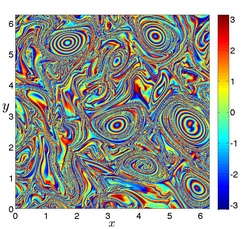
Thus, attracting, repelling and shearing material surfaces are necessarily stacked on each other, i.e., occur in continuous families. This leads to the idea of seeking LCSs in finite-time dynamical systems as exceptional material surfaces that exhibit a coherence-inducing property more strongly than any of the neighboring material surfaces. Such LCSs, defined as extrema (or more generally, stationary surfaces) for a finite-time coherence property, will indeed serve as observed centerpieces of trajectory patterns. Examples of attracting, repelling and shearing LCSs are in a direct numerical simulation of 2D turbulence are shown in Fig.2a.

LCSs vs. classical invariant manifolds

Classical invariant manifolds are invariant sets in the phase space [math]\displaystyle{ \mathcal P }[/math] of an autonomous dynamical system. In contrast, LCSs are only required to be invariant in the extended phase space. This means that even if the underlying dynamical system is autonomous, the LCSs of the system over the interval [math]\displaystyle{ I }[/math] will generally be time-dependent, acting as the evolving skeletons of observed coherent trajectory patterns. Figure 2b shows the difference between an attracting LCS and a classic unstable manifold of a saddle point, for evolving times, in an autonomous dynamical system. File:LCS vs invariant manifolds.tif

Objectivity of LCSs

Assume that the phase space of the underlying dynamical system is the material configuration space of a continuum, such as a fluid or a deformable body. For instance, for a dynamical system generated by an unsteady velocity field [math]\displaystyle{ v=v(x,t),\qquad x\in U\subset \R^3, }[/math]

the open set [math]\displaystyle{ U }[/math] of possible particle positions is a material configuration space. In this space, LCSs are material surfaces, formed by trajectories. Whether or not a material trajectory is contained in an LCS is a property that is independent of the choice of coordinates, and hence cannot depend of the observer. As a consequence, LCSs are subject to the basic objectivity (material frame-indifference) requirement of continuum mechanics. The objectivity of LCSs requires them to be invariant with respect to all possible observer changes, i.e., linear coordinate changes of the form [math]\displaystyle{ x=Q(t)y+b(t), }[/math] where [math]\displaystyle{ y \in \R^3 }[/math] is the vector of the transformed coordinates; [math]\displaystyle{ Q(t) }[/math] is an arbitrary [math]\displaystyle{ 3 \times 3 }[/math] proper orthogonal matrix representing time-dependent rotations; and [math]\displaystyle{ b(t) }[/math] is an arbitrary [math]\displaystyle{ 3 }[/math]-dimensional vector representing time-dependent translations. As a consequence, any self-consistent LCS definition or criterion should be expressible in terms of quantities that are frame-invariant. For instance, the strain rate [math]\displaystyle{ S(x,t) }[/math] and the spin tensor [math]\displaystyle{ W(x,t) }[/math] defined as [math]\displaystyle{ S(x,t)=\frac{1}{2}\left(\nabla v(x,t)+ (\nabla v(x,t))^T\right),\qquad W(x,t)=\frac{1}{2}\left(\nabla v(x,t)- (\nabla v(x,t))^T\right), }[/math] transform under Euclidean changes of frame into the quantities [math]\displaystyle{ {\tilde S}(y,t)=Q(t)^TS(x,t)Q(t),\qquad {\tilde W}(y,t)=Q(t)^TS(x,t)Q(t)-Q(t)^T{\dot Q}(t). }[/math]

A Euclidean frame change is, therefore, equivalent to a similarity transform for [math]\displaystyle{ S(x,t) }[/math], and hence an LCS approach depending only on the eigenvalues and eigenvectors of [math]\displaystyle{ S(x,t) }[/math] is automatically frame-invariant. In contrast, an LCS approach depending on the eigenvalues of [math]\displaystyle{ W(x,t) }[/math] is generally not frame-invariant.

A number of frame-dependent quantities, such as [math]\displaystyle{ \nabla v(x,t) }[/math], [math]\displaystyle{ {W}(y,t) }[/math], [math]\displaystyle{ \nabla F^t_{t_0} }[/math], as well as the averages or eigenvalues of these quantities, are routinely used in heuristic LCS detection. While such quantities may effectively mark features of the instantaneous velocity field [math]\displaystyle{ v(x,t) }[/math], the ability of these quantities to capture material mixing, transport, and coherence is limited and a priori unknown in any given frame. As an example, consider the linear unsteady fluid particle motion

[math]\displaystyle{ {\dot x}=v(x,t)=\begin{pmatrix} \sin{4t} &2+\cos{4t}\\ -2+\cos{4t}& -\sin{4t} \end{pmatrix}x, }[/math]

which is an exact solution of the two-dimensional Navier–Stokes equations. The (frame-dependent) Okubo-Weiss criterion classifies the whole domain in this flow as elliptic (vortical) because [math]\displaystyle{ q=\frac{1}{2}( {\vert S\vert}^2-{\vert W \vert}^2)\lt 0 }[/math] holds, with [math]\displaystyle{ \vert\,\cdot \,\vert }[/math] referring to the Euclidean matrix norm. As seen in Fig. 3, however, trajectories grow exponentially along a rotating line and shrink exponentially along another rotating line. In material terms, therefore, the flow is hyperbolic (saddle-type) in any frame.

Figure 3: Instantaneous streamlines and the evolution of trajectories starting from the interior of one of them in a linear solution of the Navier–Stokes equation. This dynamical system is classified as elliptic by a number of frame-dependent coherence diagnostics, such as the Okubo–Weiss criterion. (Image: Francisco Beron-Vera)

Since Newton’s equation for particle motion and the Navier–Stokes equations for fluid motion are well known to be frame-dependent, it might first seem counterintuitive to require frame-invariance for LCSs, which are composed of solutions of these frame-dependent equations. Recall, however, that the Newton and Navier–Stokes equations represent objective physical principles for material particle trajectories. As long as correctly transformed from one frame to the other, these equations generate physically the same material trajectories in the new frame. In fact, we decide how to transform the equations of motion from an [math]\displaystyle{ x }[/math]-frame to a [math]\displaystyle{ y }[/math]-frame through a coordinate change [math]\displaystyle{ x = Q(t)y+b(t) }[/math] precisely by upholding that trajectories are mapped into trajectories, i.e., by requiring [math]\displaystyle{ x(t) = Q(t)y(t)+b(t) }[/math] to hold for all times. Temporal differentiation of this identity and substitution into the original equation in the [math]\displaystyle{ x }[/math]-frame then yields the transformed equation in the [math]\displaystyle{ y }[/math]-frame. While this process adds new terms (inertial forces) to the equations of motion, these inertial terms arise precisely to ensure the invariance of material trajectories. Fully composed of material trajectories, LCSs remain invariant in the transformed equation of motion defined in the [math]\displaystyle{ y }[/math]-frame of reference. Consequently, any self-consistent LCS definition or detection method must also be frame-invariant.

Hyperbolic LCSs

Figure 4. Attracting and repelling LCSs in the extended phase space of a two-dimensional dynamical system.

Motivated by the above discussion, the simplest way to define an attracting LCS is by requiring it to be a locally strongest attracting material surface in the extended phase space [math]\displaystyle{ \mathcal P \times \mathcal I }[/math] (see. Fig. 4) . Similarly, a repelling LCS can be defined as a locally strongest repelling material surface. Attracting and repelling LCSs together are usually referred to as hyperbolic LCSs, as they provide a finite-time generalization of the classic concept of normally hyperbolic invariant manifolds in dynamical systems.

Diagnostic approach: Finite-time Lyapunov exponent (FTLE) ridges

Heuristically, one may seek initial positions [math]\displaystyle{ \mathcal M(t_0 ) }[/math] of repelling LCSs as set of initial conditions at which infinitesimal perturbations to trajectories starting from [math]\displaystyle{ \mathcal M(t_0 ) }[/math] grow locally at the highest rate relative to trajectories starting off of [math]\displaystyle{ \mathcal M(t_0 ) }[/math]. The heuristic element here is that instead of constructing a highly repelling material surface, one simply seeks points of large particle separation. Such a separation may well be due to strong shear along the set of points so identified; this set is not at all guaranteed to exert any normal repulsion on nearby trajectories.

The growth of an infinitesimal perturbation [math]\displaystyle{ {\xi}(t) }[/math] along a trajectory [math]\displaystyle{ x(t,t_0 ,x_0) }[/math] is governed by the flow map gradient [math]\displaystyle{ \nabla F^t_{t_0} }[/math]. Let [math]\displaystyle{ \epsilon{\xi}(t_0) }[/math] be a small perturbation to the initial condition [math]\displaystyle{ x_0 }[/math], with [math]\displaystyle{ 0\lt \epsilon\ll 1 }[/math], and with [math]\displaystyle{ \xi(t_0) }[/math] denoting an arbitrary unit vector in [math]\displaystyle{ \R^n }[/math]. This perturbation generally grows along the trajectory [math]\displaystyle{ x(t,t_0 ,x_0) }[/math] into the perturbation vector [math]\displaystyle{ {\xi}_\epsilon(t_1;x_0)= \nabla F^{t_1}_{t_0}(x_0)\epsilon{\xi}(t_0) }[/math]. Then the maximum relative stretching of infinitesimal perturbations at the point [math]\displaystyle{ x_0 }[/math] can be computed as

[math]\displaystyle{ \begin{align} \delta^{t_1}_{t_0}(x_0) & =\lim_{\epsilon \to 0}\frac{1}{\epsilon}\max_{\left|\xi(t_0)\right|=1}\left|\xi_{\epsilon}(t_1;x_0)\right| \\ & = \max_{\left|\xi(t_0)\right|=1}\sqrt{\left\langle \nabla F_{t_0}^{t_1}(x_0)\xi(t_0),\nabla F_{t_0}^{t_1}(x_0)\xi(t_0)\right\rangle } \\ & = \max_{\left|\xi(t_0)\right|=1}\sqrt{\left\langle \xi(t_0),C_{t_0}^{t_1}(x_0)\xi(t_0)\right\rangle } \\ \end{align} }[/math]

where [math]\displaystyle{ C^{t_1}_{t_0}=\left[ \nabla F_{t_0}^{t_1}\right]^T\nabla F_{t_0}^{t_1} }[/math] denotes the right Cauchy–Green strain tensor. One then concludes that the maximum relative stretching experienced along a trajectory starting from [math]\displaystyle{ x_0 }[/math] is just [math]\displaystyle{ \delta^{t_1}_{t_0}(x_0)=\sqrt{\lambda_n (x_0)} }[/math]. As this relative stretching tends to grow rapidly, it is more convenient to work with its growth exponent [math]\displaystyle{ (\log{\delta^{t_1}_{t_0 }})/(t_1-t_0) }[/math], which is then precisely the finite-time Lyapunov exponent (FTLE)

[math]\displaystyle{ \mathrm{FTLE}_{t_0}^{t_1}(x_0)=\frac{1}{2(t_1-t_0)}\log\lambda_{n}(x_0). }[/math]

Figure 5a. Attracting (red) and repelling (blue) LCSs extracted as FTLE ridges from a two-dimensional turbulence experiment (Image: Manikandan Mathur)

Therefore, one expects hyperbolic LCSs to appear as codimension-one local maximizing surfaces (or ridges) of the FTLE field. This expectation turns out to be justified in the majority of cases: time [math]\displaystyle{ t_0 }[/math] positions of repelling LCSs are marked by ridges of [math]\displaystyle{ \mathrm{FTLE}_{t_0}^{t_1}(x_0) }[/math]. By applying the same argument in backward time, we obtain that time [math]\displaystyle{ t_1 }[/math] positions of attracting LCSs are marked by ridges of the backward FTLE field [math]\displaystyle{ \mathrm{FTLE}_{t_1}^{t_0} }[/math].

The classic way of computing Lyapunov exponents is solving a linear differential equation for the linearized flow map [math]\displaystyle{ \nabla F^{t}_{t_0}(x_0) }[/math]. A more expedient approach is to compute the FTLE field from a simple finite-difference approximation to the deformation gradient. For example, in a three-dimenisonal flow, we launch a trajectory [math]\displaystyle{ x(t;t_0,x_0) }[/math] from any element [math]\displaystyle{ x_0 }[/math] of a grid of initial conditions. Using the coordinate representation [math]\displaystyle{ x=(x^1,x^2,x^3) }[/math] for the evolving trajectory [math]\displaystyle{ x(t;t_0,x_0) }[/math], we approximate the gradient of the flow map as [math]\displaystyle{ \nabla F_{t_0}^{t}(x_0)\approx \begin{pmatrix} \frac{x^{1}(t;t_0,x_0+\delta_1)-x^{1}(t;t_0,x_0-\delta_1)}{\left|2\delta_1\right|} & \frac{x^{1}(t;t_0,x_0+\delta_2)-x^{1}(t;t_0,x_0-\delta_2)}{\left|2\delta_2\right|} & \frac{x^{1}(t;t_0,x_0+\delta_3)-x^{1}(t;t_0,x_0-\delta_3)}{\left|2\delta_3\right|}\\ \frac{x^{2}(t;t_0,x_0+\delta_1)-x^{2}(t;t_0,x_0-\delta_1)}{\left|2\delta_1\right|} & \frac{x^{2}(t;t_0,x_0+\delta_2)-x^{2}(t;t_0,x_0-\delta_2)}{\left|2\delta_2\right|} & \frac{x^{2}(t;t_0,x_0+\delta_3)-x^{2}(t;t_0,x_0-\delta_3)}{\left|2\delta_3\right|}\\ \frac{x^{3}(t;t_0,x_0+\delta_1)-x^{3}(t;t_0,x_0-\delta_1)}{\left|2\delta_1\right|} & \frac{x^{3}(t;t_0,x_0+\delta_2)-x^{3}(t;t_0,x_0-\delta_2)}{\left|2\delta_2\right|} & \frac{x^{3}(t;t_0,x_0+\delta_3)-x^{3}(t;t_0,x_0-\delta_3)}{\left|2\delta_3\right|} \end{pmatrix} , }[/math]

Figure 5b. Attracting (blue) and repelling (red) LCSs extracted as FTLE ridges from a two-dimensional simulation of a von Karman vortex street (Image: Jens Kasten)

with a small vector [math]\displaystyle{ \delta_{i} }[/math] pointing in the [math]\displaystyle{ x^{i} }[/math] coordinate direction. For two-dimensional flows, only the first [math]\displaystyle{ 2\times 2 }[/math] minor matrix of the above matrix is relevant.

Figure 6. FTLE ridges highlight both hyperbolic LCS and shearing material lines, such as the boundaries of a riverbed in a 3D model of the New River Inlet, Onslow, North Carolina (Image: Allen Sanderson).

Issues with inferring hyperbolic LCSs from FTLE ridges

FTLE ridges have proven to be a simple and efficient tool for the visualize hyperbolic LCSs in a number of physical problems, yielding intriguing images of initial positions of hyperbolic LCSs in different applications (see, e.g., Figs. 5a-b). However, FTLE ridges obtained over sliding time windows [math]\displaystyle{ [t_0+T,t_1+T] }[/math] do not form material surfaces. Thus, ridges of [math]\displaystyle{ \mathrm{FTLE}_{t_0+T}^{t_1+T}(x_0) }[/math] under varying [math]\displaystyle{ T }[/math] cannot be used to define Lagrangian objects, such as hyperbolic LCSs. Indeed, a locally strongest repelling material surface over [math]\displaystyle{ [t_0,t_1] }[/math] will generally not play the same role over [math]\displaystyle{ [t_0+T,t_1+T] }[/math] and hence its evolving position at time [math]\displaystyle{ t_0+T }[/math] will not be a ridge for [math]\displaystyle{ \mathrm{FTLE}_{t_0+T}^{t_1+T} }[/math]. Nonetheless, evolving second-derivative FTLE ridges computed over sliding intervals of the form [math]\displaystyle{ [t_0+T,t_1+T] }[/math] have been identified by some authors broadly with LCSs. In support of this identification, it is also often argued that the material flux over such sliding-window FTLE ridges should necessarily be small.

The "FTLE ridge=LCS" identification, however, suffers form the following conceptual and mathematical problems:

• Second-derivative FTLE ridges are necessarily straight lines and hence do not exist in physical problems.
• FTLE ridges computed over sliding time windows [math]\displaystyle{ [t_0+T,t_1+T] }[/math] with a varying [math]\displaystyle{ T }[/math] are generally not Lagrangian and the flux through them is generally not small.
• In particular, a broadly referenced material flux formula for FTLE ridges is incorrect, even for straight FTLE ridges
• FTLE ridges mark hyperbolic LCS positions, but also highlight surfaces of high shear. A convoluted mixture of both types of surfaces often arises in applications (see Fig. 6 for an example).
• There are several other types LCSs (elliptic and parabolic) beyond the hyperbolic LCSs highlighted by FTLE ridges

Local variational approach: Shrink and stretch surfaces

The local variational theory of hyperbolic LCSs builds on their original definition as strongest repelling or repelling material surfaces in the flow over the time interval [math]\displaystyle{ [t_0,t_1] }[/math]. At an initial point [math]\displaystyle{ x_0 }[/math] , let [math]\displaystyle{ n_0 }[/math] denote a unit normal to an initial material surface [math]\displaystyle{ \mathcal{M}(t_0) }[/math] (cf. Fig. 6). By the invariance of material lines, the tangent space [math]\displaystyle{ T_{x_0}\mathcal{M}(t_0) }[/math] is mapped into the tangent space of [math]\displaystyle{ T_{x_1} \mathcal{M}(t_1) }[/math] by the linearized flow map [math]\displaystyle{ \nabla F_{t_0}^{t_1}(x_0) }[/math]. At the same time, the image of the normal [math]\displaystyle{ n_0 }[/math] normal under [math]\displaystyle{ \nabla F_{t_0}^{t_1}(x_0) }[/math] generally does not remain normal to [math]\displaystyle{ \mathcal{M}(t_1) }[/math]. Therefore, in addition to a normal component of length [math]\displaystyle{ \rho^{t_1}_{t_0}(x_{0,}n_0) }[/math], the advected normal also develops a tangential component of length [math]\displaystyle{ \sigma^{t_1}_{t_0}(x_0,n_0) }[/math] (cf. Fig. 7).

Figure 7. Linearized flow geometry along an evolving material surface.

If [math]\displaystyle{ \rho^{t_1}_{t_0}(x_0,n_0)\gt 1 }[/math], then the evolving material surface [math]\displaystyle{ \mathcal{M}(t) }[/math] strictly repels nearby trajectories by the end of the time interval [math]\displaystyle{ [t_0,t_1] }[/math]. Similarly, [math]\displaystyle{ \rho^{t_1}_{t_0}(x_0,n_0)\lt 1 }[/math] signals that [math]\displaystyle{ \mathcal{M}(t) }[/math] strictly attracts nearby trajectories along its normal directions. A repelling (attracting) LCS over the interval [math]\displaystyle{ [t_0,t_1] }[/math] can be defined as a material surface [math]\displaystyle{ \mathcal{M}(t) }[/math] whose net repulsion [math]\displaystyle{ \rho^{t_1}_{t_0}(x_0,n_0) }[/math] is pointwise maximal (minimal) with respect to perturbations of the initial normal vector field [math]\displaystyle{ n_0 }[/math]. As earlier, we refer to repelling and attracting LCSs collectively as hyperbolic LCSs.

Solving these local extremum principles for hyperbolic LCSs in two and three dimensions yields unit normal vector fields to which hyperbolic LCSs should everywhere be tangent. The existence of such normal surfaces also requires a Frobenius-type integrability condition in the three-dimensional case. All these results can be summarized as follows:

Hyperbolic LCS conditions from local variational theory in dimensions n=2 and n=3

LCS	Normal vector field of [math]\displaystyle{ \mathcal M(t_0) }[/math] for [math]\displaystyle{ n=2,3 }[/math]	ODE for [math]\displaystyle{ \mathcal M(t_0) }[/math] for n=2	Frobenius-type PDE for [math]\displaystyle{ \mathcal M(t_0) }[/math] for n=3
Attracting	[math]\displaystyle{ \xi_1 (x_0) }[/math]	[math]\displaystyle{ x^{\prime}_0 =\xi_2(x_0) }[/math] (stretch lines)	[math]\displaystyle{ \left\langle \nabla\times\xi_1(x_0),\xi_1(x_0)\right\rangle =0 }[/math] (stretch surfaces)
Repelling	[math]\displaystyle{ \xi_n (x_0) }[/math]	[math]\displaystyle{ x^{\prime}_0 =\xi_1(x_0) }[/math] (shrink lines)	[math]\displaystyle{ \left\langle \nabla\times\xi_3(x_0),\xi_3(x_0)\right\rangle =0 }[/math] (shrink surfaces)

Repelling LCSs are obtained as most repelling shrink lines, starting from local maxima of [math]\displaystyle{ \lambda_2 (x_0) }[/math]. Attracting LCSs are obtained as most attracting stretch lines, starting from local minima of [math]\displaystyle{ \lambda_1 (x_0) }[/math]. These starting points serve are initial positions of exceptional saddle-type trajectories in the flow. An example of the local variational computation of a repelling LCS is shown in FIg. 8. The computational algorithm is available in LCS Tool. File:Repelling LCS for double gyre.tiff

In 3D flows, instead of solving the Frobenius PDE (see table above) for hyperbolic LCSs, an easier approach is to construct intersections of hyperbolic LCSs with select 2D planes, and fit a surface numerically to a large number of such intersection curves. Let us denote the unit normal of a 2D plane [math]\displaystyle{ \Pi }[/math] by [math]\displaystyle{ n_\Pi }[/math]. The intersection curve of a 2D repelling LCS surface with the plane [math]\displaystyle{ \Pi }[/math] is normal to both [math]\displaystyle{ n_\Pi }[/math] and to the unit normal [math]\displaystyle{ \xi_3(x_0) }[/math] of the LCS. As a consequence, an intersection curve [math]\displaystyle{ x_0(s) }[/math] satisfies the ODE

[math]\displaystyle{ x^{\prime}_0 =\xi_3(x_0)\times n_\Pi, }[/math]

whose trajectories we refer to as reduced shrink lines. (Strictly speaking, this equation is not an ordinary differential equation, given that its right-hand side is not a vector field, but a direction field, which is generally not globally orientable). Intersections of hyperbolic LCSs with [math]\displaystyle{ \Pi }[/math] are fastest contracting reduced shrink lines. Determining such shrink lines in a smooth family of nearby [math]\displaystyle{ \Pi }[/math] planes, then fitting a surface to the curve family so obtained yields a numerical approximation of a 2D repelling LCS.

Global variational approach: Shrink- and stretchlines as null-geodesics

A general material surface experiences shear and strain in its deformation, both of which depend continuously on initial conditions by the continuity of the map [math]\displaystyle{ F^t_{t_0} }[/math]. The averaged strain and shear within a strip of [math]\displaystyle{ \mathcal O(\epsilon) }[/math]-close material lines, therefore, typically show [math]\displaystyle{ \mathcal O(\epsilon) }[/math] variation within such a strip. The two-dimensional geodesic theory of LCSs seeks exceptionally coherent locations where this general trend fails, resulting in an order of magnitude smaller variability in shear or strain than what is normally expected across an [math]\displaystyle{ \mathcal O(\epsilon) }[/math] strip. Specifically, the geodesic theory searches for LCSs as special material lines around which [math]\displaystyle{ \mathcal O(\epsilon) }[/math] material strips show no [math]\displaystyle{ \mathcal O(\epsilon) }[/math] variability either in the material-line averaged shear (Shearless LCSs) or in the material-line averaged strain (Strainless or Elliptic LCSs). Such LCSs turn out to be null-geodesics of appropriate metric tensors defined by the deformation field—hence the name of this theory.

Shearless LCSs are found to be null-geodesics of a Lorentzian metric tensor [math]\displaystyle{ D_{t_0}^{t_1} }[/math] defined as

[math]\displaystyle{ D_{t_0}^{t_1}(x_0)=\frac{1}{2}\left[C_{t_0}^{t_1}(x_0)\Omega-\Omega C_{t_0}^{t_1}(x_0)\right], \qquad \Omega = \begin{pmatrix} 0 & -1 \\ 1 & 0 \\ \end{pmatrix} . }[/math]

Such null-geodesics can be proven to be tensorlines of the Cauchy–Green strain tensor, i.e., are tangent to the direction field formed by the strain eigenvector fields [math]\displaystyle{ \xi_i(x_0) }[/math]. Specifically, repelling LCSs are trajectories of [math]\displaystyle{ x_0^{\prime} =\xi_1(x_0) }[/math] starting from local maxima of the [math]\displaystyle{ \lambda_2(x_0) }[/math] eigenvalue field. Similarly, attracting LCSs are trajectories of [math]\displaystyle{ x_0^{\prime}=\xi_2(x_0) }[/math] starting from local minims of the [math]\displaystyle{ \lambda_1(x_0) }[/math] eigenvalue field. This agrees with the conclusion of the local variational theory of LCSs. The geodesic approach, however, also sheds more light on the robustness of hyperbolic LCSs: hyperbolic LCSs only prevail as stationary curves of the averaged shear functional under variations that leave their endpoints fixed. This is to be contrasted with parabolic LCSs (see below), which are also shearless LCSs but prevail as stationary curves to the shear functional even under arbitrary variations. As a consequence, individual trajectories are objective, and statements about the coherent structures they form should also be objective.

A sample application is shown in Fig. 9, where the sudden appearance of a hyperbolic core (strongest attracting part of a stretchline) within the oil spill caused the notable Tiger-Tail instability in the shape of the oil spill.

Elliptic LCSs

Elliptc LCSs are closed and nested material surfaces that act as building blocks of the Lagrangian equivalents of vortices, i.e., rotation-dominated regions of trajectories that generally traverse the phase space without substantial stretching or folding. They mimic the behavior of Kolmogorov–Arnold–Moser (KAM) tori that form elliptic regions in Hamiltonian systems. There coherence can be approached either through their homogeneous material rotation or through their homogeneous stretching properties.

Rotational coherence from the polar rotation angle (PRA)

As a simplest approach to rotational coherence, one may define an elliptic LCS as a tubular material surface along which small material volumes complete the same net rotation over the time intervall [math]\displaystyle{ [t_0 ,t_1] }[/math] of interest. A challenge in that in each material volume element, all individual material fibers (tangent vectors to trajectories) perform different rotations.

To obtain a well-defined bulk rotation for each material element, one may employ the unique left and right polar decompositions of the flow gradient in the form

[math]\displaystyle{ \nabla F^{t_1}_{t_0}=R^{t_1}_{t_0}U^{t_1}_{t_0}=V^{t_1}_{t_0}R^{t_1}_{t_0}, }[/math] where the proper orthogonal tensor [math]\displaystyle{ R^{t_1}_{t_0} }[/math] is called the rotation tensor and the symmetric, positive definite tensors [math]\displaystyle{ U^{t_1}_{t_0},V^{t_1}_{t_0} }[/math] are called the left stretch tensor and right stretch tensor, respectively.

Since the Cauchy–Green strain tensor can be written as [math]\displaystyle{ C^{t_1}_{t_0}=[\nabla F^{t_1}_{t_0}]^T\nabla F^{t_1}_{t_0}=U^{t_1}_{t_0}U^{t_1}_{t_0}=V^{t_1}_{t_0}V^{t_1}_{t_0}, }[/math] the local material straining described by the eigenvalues and eigenvectors of [math]\displaystyle{ C^{t_1}_{t_0} }[/math] are fully captured by the singular values and singular vectors of the stretch tensors. The remaining factor in the deformation gradient is represented by [math]\displaystyle{ R^{t_1}_{t_0} }[/math], interpreted as the bulk solid-body rotation component of volume elements. In planar motions, this rotation is defined relative to the normal of the plane. In three dimensions, the rotation is defined relative to the axis defined by the eigenvector of [math]\displaystyle{ R^{t_1}_{t_0} }[/math] corresponding to its unit eigenvalue. In higher-dimensional flows, the rotation tensor cannot be viewed as a rotation about a single axis.

Figure 10a. Elliptic LCSs revealed by closed level curves of the PRA distribution in a two-dimensional turbulence simulation. (Image: Mohammad Farazmand)

Figure 10b. Elliptic LCSs revealed by closed level curves of the PRA distribution in the steady ABC flow. (Image: Mohammad Farazmand)

In two and three dimensions, therefore, there exists a polar rotation angle (PRA) [math]\displaystyle{ \theta_{t_0}^{t_1}(x_0) }[/math] that characterises the material rotation generated by [math]\displaystyle{ R^{t_1}_{t_0} }[/math] for a volume element centered at the initial condition [math]\displaystyle{ x_0 }[/math]. This PRA is well-defined up to multiples of [math]\displaystyle{ 2\pi }[/math]. For two-dimensional flows, the PRA can be computed from the invariants of [math]\displaystyle{ C^{t_1}_{t_0} }[/math] using the formulas

[math]\displaystyle{ \begin{align} \cos\theta_{t_0}^{t_1}&=\frac{\langle \xi_{i},\nabla F^{t_1}_{t_0}\xi_{i}\rangle }{\sqrt{\lambda_{i}}},\quad i=1\,\,or\,\,\,2,\\ \sin\theta_{t_0}^{t_1}&=\left(-1\right)^{j}\frac{\langle \xi_{i},\nabla F^{t_1}_{t_0}\xi_{j}\rangle }{\sqrt{\lambda_{j}}},\qquad (i,j)=(1,2)\,\,or\,\,(2,1),\\ \end{align} }[/math]

which yield a four-quadrant version of the PRA via the formula

[math]\displaystyle{ \theta_{t_0}^{t}=\left[1-{\rm sign\,}\left(\sin\theta_{t_0}^{t}\right)\right]\pi+{\rm sign\,}\left(\sin\theta_{t_0}^{t}\right)\cos^{-1}\left(\cos\theta_{t_0}^{t}\right). }[/math]

For three-dimensional flows, the PRA can again be computed from the invariants of [math]\displaystyle{ C^{t_1}_{t_0} }[/math] from the formulas

[math]\displaystyle{ \begin{align} \cos\theta_{t_0}^{t}&=\frac{1}{2}\left(\sum_{i=1}^{3}\frac{\left\langle \xi_{i},\nabla F^{t_1}_{t_0}\xi_{i}\right\rangle }{\sqrt{\lambda_{i}}}-1\right),\\ \sin\theta_{t_0}^{t} &=\frac{\left\langle \xi_{i},\nabla F^{t_1}_{t_0}\xi_{j}\right\rangle -\left\langle \xi_{j},\nabla F^{t_1}_{t_0}\xi_{i}\right\rangle }{2\epsilon_{ijk}e_{k}},\qquad i\neq j, \end{align} }[/math] where [math]\displaystyle{ \epsilon_{ijk} }[/math] is the Levi-Civita symbol, [math]\displaystyle{ \mathbf{e}=\left\{ e_{k}\right\} }[/math] is the eigenvector corresponding to the unit eigenvector of the matrix [math]\displaystyle{ \left[K_{t_0}^{t}\right]_{jk}=\left\langle \xi_{j},\nabla F^{t_1}_{t_0}\xi_{k}\right\rangle/{\sqrt{\lambda_{k}}} }[/math].

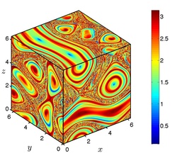
The time [math]\displaystyle{ t_0 }[/math] positions of elliptic LCSs are visualized as tubular level sets of the PRA distribution [math]\displaystyle{ \theta_{t_0}^{t} }[/math]. In two-dimensions, therefore, (polar) elliptic LCSs are simply closed level curves of the PRA, which turn out to be objective. In three dimensions, (polar) elliptic LCSs are toroidal or cylindrical level surfaces of the PRA, which are, however, not objective and hence will generally change in rotating frames. Coherent Lagrangian vortex boundaries can be visualized as outermost members of nested families of elliptic LCSs. Two- and three-dimensional examples of elliptic LCS revealed by tubular level surfaces of the PRA are shown in Fig. 10a-b.

Rotational coherence from the Lagrangian-averaged vorticity deviation (LAVD)

The level sets of the PRA are objective in two dimensions but not in three dimensions. An additional shortcoming of the polar rotation tensor is its dynamical inconsistency: polar rotations computed over adjacent sub-intervals of a total deformation do not sum up to the rotation computed for the full-time interval of the same deformation. Therefore, while [math]\displaystyle{ R_{t_0}^{t_1} }[/math] is the closest rotation tensor to [math]\displaystyle{ \nabla F^{t_1}_{t_0} }[/math] in the [math]\displaystyle{ L^2 }[/math] norm over a fixed time interval [math]\displaystyle{ [t_0,t_1] }[/math], these piecewise best fits do not form a family of rigid-body rotations as [math]\displaystyle{ t_0 }[/math] and [math]\displaystyle{ t_1 }[/math] are varied. For this reason, rotations predicted by the polar rotation tensor over varying time intervals divert from the experimentally observed mean material rotation of fluid elements.

Figure 11a: Rotationally coherent mesoscale eddy boundaries in the ocean at time t0 = November 11, 2006, identified from satellite-based surface velocities, using the integration time t1-t0=90 days. The boundaries are identified as outermost closed contours of the LAVD with small convexity deficiency. Also shown in the background is the contour plot of the LAVD field for reference. (Image: Alireza Hadjighasem)

Figure 11b: Materially advected rotationally coherent mesoscale eddy boundaries and eddy centers in the ocean, along with representative inertial particle trajectories initialised on the eddy boundaries. The eddy centers are obtained as local maxima of the LAVD field. As can be proven mathematically, heavy particles (cyan) converge to the centers of anti-cyclonic (clockwise) eddies. Light particles (black) converge to the centers of cyclonic (clockwise) eddies. (Movie: Alireza Hadjighasem)

An alternative to the classic polar decomposition provides a resolution to both the non-objectivity and the dynamic inconsistency issue. Specifically, the Dynamic Polar Decomposition (DPD) of the deformation gradient is also of the form

[math]\displaystyle{ \nabla F^{t}_{t_0}=O_{t_0}^{t}M_{t_0}^{t}=N_{t_0}^{t}O_{t_0}^{t}, }[/math]

where the proper orthogonal tensor [math]\displaystyle{ O^{t}_{t_0} }[/math] is the dynamic rotation tensor and the non-singular tensors [math]\displaystyle{ M^{t}_{t_0},N^{t}_{t_0} }[/math] are the left dynamic stretch tensor and right dynamic stretch tensor, respectively. Just as the classic polar decomposition, the DPD is valid in any finite dimension. Unlike the classic polar decomposition, however, the dynamic rotation and stretch tensors are obtained from solving linear differential equations, rather than from matrix manipulations. In particular, [math]\displaystyle{ O_{t_0}^{t}=\nabla_{a_0}a(t) }[/math] is the deformation gradient of the purely rotational flow

[math]\displaystyle{ \dot{a}=W\left(x(t;x_0),t\right)a, }[/math]

and [math]\displaystyle{ M_{t_0}^{t}=\nabla_{b_0}b(t) }[/math] is the deformation gradient of the purely straining flow

[math]\displaystyle{ \dot{b} = O_{t}^{t_0}S\left(x(t;x_0),t\right)O_{t_0}^{t} b. }[/math].

The dynamic rotation tensor [math]\displaystyle{ O_{t_0}^{t} }[/math] can further be factorized into two deformation gradients: one for a spatially uniform (rigid-body) rotation, and one that deviates from this uniform rotation:

[math]\displaystyle{ O_{t_0}^{t}=\Phi_{t_0}^{t}\Theta_{t_0}^{t}. }[/math]

As a spatially independent rigid-body rotation, the proper orthogonal relative rotation tensor [math]\displaystyle{ \Phi_{t_0}^{t}=\partial_{\alpha_0} \alpha(t) }[/math] is dynamically consistent, serving as the deformation gradient of the relative rotation flow

[math]\displaystyle{ \dot{\alpha}=\left[W\left(x(t;x_0),t\right)-\bar{W}\left(t\right)\right]\alpha. }[/math]

In contrast, the proper orthogonal mean rotation tensor [math]\displaystyle{ \Theta_{t_0}^{t}=D_{\beta_0}\beta(t) }[/math] is the deformation gradient of the mean-rotation flow

[math]\displaystyle{ \dot{\beta}=\Phi_{t}^{t_0}\bar{W}\left(t\right)\Phi_{t_0}^{t}\beta. }[/math] The dynamic consistency of [math]\displaystyle{ \Phi_{t_0}^{t} }[/math] implies that the total angle swept by [math]\displaystyle{ \Phi_{t_0}^{t} }[/math] around its own axis of rotation is dynamically consistent. This intrinsic rotation angle [math]\displaystyle{ \psi_{t_0}^{t}(x_0) }[/math] is also objective, and turns out to equal to one half of the Lagrangian-averaged vorticity deviation (LAVD). The LAVD is defined as the trajectory-averaged magnitude of the deviation of the vorticity from its spatial mean. With the vorticity [math]\displaystyle{ \omega (x,t)=\nabla\times v(x,t) }[/math] and its spatial mean [math]\displaystyle{ \bar{\omega}(t)=\frac{\int_{U(t)}\omega(x,t)\,dV}{\mathrm{vol}\,(U(t))}, }[/math] the LAVD over a time interval [math]\displaystyle{ [t_0,t_1] }[/math] therefore takes the form [math]\displaystyle{ \mathrm{LAVD}_{t_0}^{t_1}(x_0):=\int_{t_0}^{t_1}\left|\omega(x(s;x_0),s)-\bar{\omega}(s)\right|\,ds, }[/math]

with [math]\displaystyle{ U(t) }[/math] denoting the (possibly time-varying) domain of definition of the velocity field [math]\displaystyle{ v(x,t) }[/math]. This result applies both in two- and three dimensions, and enables the computation of a well-defined, objective and dynamically consistent material rotation angle along any trajectory.

Figure 11c: A rotationally coherent mesoscale eddy (yellow) in the Southern Ocean State Estimate (SOSE) ocean model at t0 = May 15, 2006, computed as a tubular LAVD level surface over t1-t0=120 days. Also shown are nearby LAVD level surfaces to illustrate the rotational incoherence outside the eddy. (Image: Alireza Hadjighasem)

Outermost complex tubular level curves of the LAVD define initial positions of rotationally coherent material vortex boundaries in two-dimensional unsteady flows (see Fig. 11a). By construction, these boundaries may exhibit transverse filamentation, but any developing filament keeps rotating with the boundary, without global transverse departure form the material vortex. (Exceptions are inviscid flows where such a global departure of LAVD level surfaces from a vortex is possible as fluid elements preserve their material rotation rate for all times). Remarkably, centers of rotationally coherent vortices (defined by local maxima of the LAVD field) can be proven to be the observed centers of attraction or repulsion for finite-size (inertial) particle motion in geophysical flows (see Fig. 11b). In three-dimensional flows, tubular level surfaces of the LAVD define initial positions of two-dimensional eddy boundary surfaces (see Fig. 11c) that remain rotationally coherent over a time intcenter|erval [math]\displaystyle{ [t_0,t_1] }[/math] (see Fig. 11d).

Fig. 11c Material advection of a rotationally coherent Lagrangian vortex and its core in the 3D SOSE model data set. (Animation: Alireza Hadjighasem)

Stretching-based coherence from a local variational approach: Shear surfaces

The local variational theory of elliptic LCSs targets material surfaces that locally maximize material shear over the finite time interval [math]\displaystyle{ [t_0,t_1] }[/math] of interest. This means that at initial point each point [math]\displaystyle{ x_0 \in \mathcal M(t_0) }[/math] of an elliptic LCS [math]\displaystyle{ \mathcal M(t) }[/math], the tangent space [math]\displaystyle{ T_{x_0} \mathcal M(t_0) }[/math] is the plane along which the local Lagrangian shear [math]\displaystyle{ \sigma^{t_1}_{t_0}(x_0) }[/math] is maximal (cf. Fig 7).

Introducing the two-dimensional shear vector field [math]\displaystyle{ \eta^{\pm}(x_0):=\sqrt{\frac{\lambda_2(x_0)-1}{\lambda_2(x_0)-\lambda_1(x_0)}}\xi_1(x_0)\pm\sqrt{\frac{1-\lambda_1(x_0)}{\lambda_2(x_0)-\lambda_1(x_0)}}\xi_2(x_0), }[/math] and the three-dimensional shear normal vector field [math]\displaystyle{ n_{\pm}(x_0)=\sqrt{\frac{\sqrt{\lambda_1(x_0)}}{\sqrt{\lambda_1(x_0)}+\sqrt{\lambda_3(x_0)}}}\xi_1(x_0)\pm\sqrt{\frac{\sqrt{\lambda_3(x_0)}}{\sqrt{\lambda_1(x_0)}+\sqrt{\lambda_3(x_0)}}}\xi_3(x_0), }[/math]

the criteria for two- and three-dimensional elliptic LCSs can be summarized as follows:

Ellipitic LCS conditions from local variational theory in dimensions n=2 and n=3

LCS	Normal vector field of [math]\displaystyle{ \mathcal M(t_0) }[/math] for n=3	ODE for [math]\displaystyle{ \mathcal M(t_0) }[/math] for n=2	Frobenius-type PDE for [math]\displaystyle{ \mathcal M(t_0) }[/math] for n=3
Elliptic	[math]\displaystyle{ n_{\pm}(x_0) }[/math]	[math]\displaystyle{ x^{\prime}_0 =\eta^{\pm}(x_0) }[/math] (shear lines)	[math]\displaystyle{ \langle \nabla\times n_{\pm}(x_0),n_{\pm}(x_0)\rangle =0 }[/math] (shear surfaces)

For 3D flows, as in the case of hyperbolic LCSs, solving the Frobenius PDE can be avoided. Instead, one can construct intersections of a tubular elliptic LCS with select 2D planes, and fit a surface numerically to a large number of these intersection curves. As for hyperbolic LCSs above, let us denote the unit normal of a 2D plane [math]\displaystyle{ \Pi }[/math] by [math]\displaystyle{ n_\Pi }[/math]. Again, the intersection curves of elliptic LCSs with the plane [math]\displaystyle{ \Pi }[/math] are normal to both [math]\displaystyle{ n_\Pi }[/math] and to the unit normal [math]\displaystyle{ n_{\pm}(x_0) }[/math] of the LCS. As a consequence, an intersection curve [math]\displaystyle{ x_0(s) }[/math] satisfies the reduced shear ODE [math]\displaystyle{ x^{\prime}_0 =n_{\pm}(x_0)\times n_\Pi, }[/math] whose trajectories we refer to as reduced shear lines. (Strictly speaking, the reduced shear ODE is not an ordinary differential equation, given that its right-hand side is not a vector field, but a direction field, which is generally not globally orientable). Intersections of tubular elliptic LCSs with [math]\displaystyle{ \Pi }[/math] are limit cycles of the reduced shear ODE. Determining such limit cycles in a smooth family of nearby [math]\displaystyle{ \Pi }[/math] planes, then fitting a surface to the limit cycle family yields a numerical approximation for 2D shear surface. A three-dimensional example of this local variational computation of an elliptic LCS is shown in Fig. 11. File:VARI LCS 3D ABC.tiff

Stretching-based coherence from a global variational approach: lambda-lines

Figure 13. Nested family of elliptic LCSs, obtained as [math]\displaystyle{ \lambda }[/math]-lines, forming transport barriers around the Great Red Spot (GRS) of Jupiter. These LCSs were identified in a two-dimensional, unsteady velocity field reconstructed from a video footage of Jupiter. The color indicates the corresponding values of the parameter [math]\displaystyle{ \lambda }[/math]. Also shown is the perfectly coherent ([math]\displaystyle{ \lambda=1 }[/math]-line) bounding the core of the GRS, as well as the outermost elliptic LCS serving as the Lagrangian vortex boundary of the GRS. Image:Alireza Hadjighasem.

As noted above under hyperbolic LCSs, a global variational approach has been developed in two dimensions to capture elliptic LCSs as closed stationary curves of the material-line-averaged Lagrangian strain functional. Such curves turn out to be closed null-geodesics of the generalized Green–Lagrange strain tensor family [math]\displaystyle{ \frac{1}{2}(C^{t_1}_{t_0}-\lambda I) }[/math], where [math]\displaystyle{ \lambda \gt 0 }[/math] is a positive parameter (Lagrange multiplier). The closed null-geodesics can be shown to coincide with limit cycles of the family of direction fields

[math]\displaystyle{ \eta^{\pm}_\lambda(x_0):=\sqrt{\frac{\lambda_2(x_0)-\lambda^2}{\lambda_2(x_0)-\lambda_1(x_0)}}\xi_1(x_0)\pm\sqrt{\frac{\lambda^2-\lambda_1(x_0)}{\lambda_2(x_0)-\lambda_1(x_0)}}\xi_2(x_0), }[/math]

Note that for [math]\displaystyle{ \lambda =1 }[/math], the direction field [math]\displaystyle{ \eta^{\pm}_\lambda(x_0 }[/math] coincides with the direction field [math]\displaystyle{ \eta^{\pm}(x_0 }[/math] for shearlines obtained above from the local variational theory of LCSs.

Trajectories of [math]\displaystyle{ \eta^{\pm}_\lambda }[/math] are referred to as [math]\displaystyle{ \lambda }[/math]-lines. Remarkably, they are initial positions of material lines that are infinitesimally uniformly stretching under the flow map [math]\displaystyle{ F^{t_1}_{t_0} }[/math]. Specifically, any subset of a [math]\displaystyle{ \lambda }[/math]-line is stretched by a factor of [math]\displaystyle{ \lambda }[/math] between the times [math]\displaystyle{ t_0 }[/math] and [math]\displaystyle{ t_1 }[/math]. As an example, Fig. 13 shows elliptic LCSs identified as closed [math]\displaystyle{ \lambda }[/math]-lines within the Great Red Spot of Jupiter.

Parabolic LCSs

Parabolic LCSs are shearless material surfaces that delineate cores of jet-type sets of trajectories. Such LCSs are characterized by both low stretching (because they are inside a non-stretching structure), but also by low shearing (because material shearing is minimal in jet cores).

Diagnostic approach: Finite-time Lyapunov exponents (FTLE) trenches

Since both shearing and stretching are as low as possible along a parabolic LCS, one may seek initial positions of such material surfaces as trenches of the FTLE field [math]\displaystyle{ FTLE^{t_1}_{t_0}(x_0) }[/math]. A geophysical example of a parabolic LCS (generalized jet core) revealed as a trench of the FTLE field is shown in Fig. 14a.

Global variational approach: Heteroclinic chains of null-geodesics

In two dimensions, parabolic LCSs are also solutions of the global shearless variational principle described above for hyperbolic LCSs. As such, parabolic LCSs are composed of shrink lines and stretch lines that represent geodesics of the Lorentzian metric tensor [math]\displaystyle{ D^{t_1}_{t_0} }[/math]. In contrast to hyperbolic LCSs, however, parabolic LCSs satisfy more robust boundary conditions: they remain stationary curves of the material-line-averaged shear functional even under variations to their endpoints. This explains the high degree of robustness and observability that jet cores exhibit in mixing. This is to be contrasted with the highly sensitive and fading footprint of hyperbolic LCSs away from strongly hyperbolic regions in diffusive tracer patterns.

Under variable endpoint boundary conditions, initial positions of parabolic LCSs turn out to be alternating chains of shrink lines and stretch lines that connect singularities of these line fields. These singularities occur at points where [math]\displaystyle{ \lambda_1(x_0)=\lambda_2(x_0) }[/math], and hence no infinitesimal deformation takes place between the two time instances [math]\displaystyle{ t_0 }[/math] and [math]\displaystyle{ t_1 }[/math]. Fig. 14b shows an example of parabolic LCSs in Jupiter's atmosphere, located using this variational theory. The chevron-type shapes forming out of circular material blobs positioned along the jet core is characteristic of tracer deformation near parabolic LCSs.

Figure 14b: Parabolic LCSs delineating unsteady Lagrangian jet cores in the atmosphere of Jupiter. Also shown is the evolution of the elliptic LCS marking the boundary of the Great Red Spot. Video:Alireza Hadjighasem.

Software packages for LCS computations

Particle advection and Finite-Time Lyapunov Exponent calculation:

• ManGen (source code)
• LCS MATLAB Kit (source code)
• FlowVC (source code)
• cuda_ftle (source code)
• CTRAJ
• Newman (source code)
• FlowTK (source code)

See also

• Turbulence
• Chaos theory
• Dynamical systems theory
• Spectral submanifold
• Eulerian coherent structure
• Coherent turbulent structure

Further reading

• Salman, H.; Hesthaven, J. S.; Warburton, T.; Haller, G. (2006). "Predicting transport by Lagrangian coherent structures with a high-order method". Theoretical and Computational Fluid Dynamics 21 (1): 39–58. doi:10.1007/s00162-006-0031-0. Bibcode: 2007ThCFD..21...39S. http://infoscience.epfl.ch/record/190478. 
• Green, M. A.; Rowley, C. W.; Haller, G. (2007). "Detection of Lagrangian coherent structures in three-dimensional turbulence". Journal of Fluid Mechanics 572: 111–120. doi:10.1017/S0022112006003648. Bibcode: 2007JFM...572..111G.

References

- ↑ 1.0 1.1 Haller, G. (2023). Transport Barriers and Coherent Structures in Flow Data. Cambridge University Press. ISBN 978-1-009-22519-9. https://www.cambridge.org/core/books/transport-barriers-and-coherent-structures-in-flow-data/F5A59AA49D5907C11B27276D036947D2#fndtn-information.
- ↑ 2.0 2.1 2.2 2.3 2.4 2.5 2.6 2.7 Haller, G.; Yuan, G. (2000). "Lagrangian coherent structures and mixing in two-dimensional turbulence". Physica D: Nonlinear Phenomena 147 (3–4): 352. doi:10.1016/S0167-2789(00)00142-1. Bibcode: 2000PhyD..147..352H.
- ↑ Peacock, T.; Haller, G. (2013). "Lagrangian coherent structures: The hidden skeleton of fluid flows". Physics Today 66 (2): 41. doi:10.1063/PT.3.1886. Bibcode: 2013PhT....66b..41P.
- ↑ 4.00 4.01 4.02 4.03 4.04 4.05 4.06 4.07 4.08 4.09 4.10 4.11 Haller, G. (2015). "Lagrangian Coherent Structures". Annual Review of Fluid Mechanics 47 (1): 137–162. doi:10.1146/annurev-fluid-010313-141322. Bibcode: 2015AnRFM..47..137H.
- ↑ Bozorgmagham, A. E.; Ross, S. D.; Schmale, D. G. (2013). "Real-time prediction of atmospheric Lagrangian coherent structures based on forecast data: An application and error analysis". Physica D: Nonlinear Phenomena 258: 47–60. doi:10.1016/j.physd.2013.05.003. Bibcode: 2013PhyD..258...47B.
- ↑ Bozorgmagham, A. E.; Ross, S. D. (2015). "Atmospheric Lagrangian coherent structures considering unresolved turbulence and forecast uncertainty". Communications in Nonlinear Science and Numerical Simulation 22 (1–3): 964–979. doi:10.1016/j.cnsns.2014.07.011. Bibcode: 2015CNSNS..22..964B.
- ↑ Olascoaga, M. J.; Haller, G. (2012). "Forecasting sudden changes in environmental pollution patterns". Proceedings of the National Academy of Sciences 109 (13): 4738–4743. doi:10.1073/pnas.1118574109. PMID 22411824. Bibcode: 2012PNAS..109.4738O.
- ↑ Nencioli, F.; d'Ovidio, F.; Doglioli, A. M.; Petrenko, A. A. (2011). "Surface coastal circulation patterns by in-situ detection of Lagrangian coherent structures". Geophysical Research Letters 38 (17): n/a. doi:10.1029/2011GL048815. Bibcode: 2011GeoRL..3817604N.
- ↑ Olascoaga, M. J.; Beron-Vera, F. J.; Haller, G.; Triñanes, J.; Iskandarani, M.; Coelho, E. F.; Haus, B. K.; Huntley, H. S. et al. (2013). "Drifter motion in the Gulf of Mexico constrained by altimetric Lagrangian coherent structures". Geophysical Research Letters 40 (23): 6171. doi:10.1002/2013GL058624. Bibcode: 2013GeoRL..40.6171O.
- ↑ Huhn, F.; von Kameke, A.; Pérez-Muñuzuri, V.; Olascoaga, M. J.; Beron-Vera, F. J. (2012). "The impact of advective transport by the South Indian Ocean Countercurrent on the Madagascar plankton bloom". Geophysical Research Letters 39 (6): n/a. doi:10.1029/2012GL051246. Bibcode: 2012GeoRL..39.6602H.
- ↑ Peng, J.; Peterson, R. (2012). "Attracting structures in volcanic ash transport". Atmospheric Environment 48: 230–239. doi:10.1016/j.atmosenv.2011.05.053. Bibcode: 2012AtmEn..48..230P.
- ↑ Tallapragada, P.; Ross, S. D.; Schmale, D. G. (2011). "Lagrangian coherent structures are associated with fluctuations in airborne microbial populations". Chaos: An Interdisciplinary Journal of Nonlinear Science 21 (3): 033122. doi:10.1063/1.3624930. PMID 21974657. Bibcode: 2011Chaos..21c3122T. http://hdl.handle.net/10919/24411.
- ↑ Ali, S.; Shah, M. (2007). "A Lagrangian Particle Dynamics Approach for Crowd Flow Segmentation and Stability Analysis". 2007 IEEE Conference on Computer Vision and Pattern Recognition. p. 1. doi:10.1109/CVPR.2007.382977. ISBN 978-1-4244-1179-5.
- ↑ Ramos, A. G.; García-Garrido, V. J.; Mancho, A. M.; Wiggins, S.; Coca, J.; Glenn, S.; Schofield, O.; Kohut, J. et al. (2018-03-15). "Lagrangian coherent structure assisted path planning for transoceanic autonomous underwater vehicle missions" (in en). Scientific Reports 8 (1): 4575. doi:10.1038/s41598-018-23028-8. ISSN 2045-2322. PMID 29545527. Bibcode: 2018NatSR...8.4575R.
- ↑ Tew Kai, Emilie; Rossi, Vincent; Sudre, Joel; Weimerskirch, Henri; Lopez, Cristobal; Hernandez-Garcia, Emilio; Marsac, Francis; Garçon, Veronique (2009-05-19). "Top marine predators track Lagrangian coherent structures" (in en). Proceedings of the National Academy of Sciences 106 (20): 8245–8250. doi:10.1073/pnas.0811034106. ISSN 0027-8424. PMID 19416811. Bibcode: 2009PNAS..106.8245T.
- ↑ Haller, G. (2001). "Lagrangian structures and the rate of strain in a partition of two-dimensional turbulence". Physics of Fluids 13 (11): 3365–3385. doi:10.1063/1.1403336. Bibcode: 2001PhFl...13.3365H.
- ↑ Haller, G. (2005). "An objective definition of a vortex". Journal of Fluid Mechanics 525: 1–26. doi:10.1017/S0022112004002526. Bibcode: 2005JFM...525....1H.
- ↑ Haller, G. (2001). "Distinguished material surfaces and coherent structures in three-dimensional fluid flows". Physica D: Nonlinear Phenomena 149 (4): 248–277. doi:10.1016/S0167-2789(00)00199-8. Bibcode: 2001PhyD..149..248H.
- ↑ Mathur, M.; Haller, G.; Peacock, T.; Ruppert-Felsot, J.; Swinney, H. (2007). "Uncovering the Lagrangian Skeleton of Turbulence". Physical Review Letters 98 (14). doi:10.1103/PhysRevLett.98.144502. PMID 17501277. Bibcode: 2007PhRvL..98n4502M.
- ↑ 20.0 20.1 Haller, G. (2002). "Lagrangian coherent structures from approximate velocity data". Physics of Fluids 14 (6): 1851–1861. doi:10.1063/1.1477449. Bibcode: 2002PhFl...14.1851H.
- ↑ Kasten, J.; Petz, C.; Hotz, I.; Hege, H. C.; Noack, B. R.; Tadmor, G. (2010). "Lagrangian feature extraction of the cylinder wake". Physics of Fluids 22 (9): 091108–091108–1. doi:10.1063/1.3483220. Bibcode: 2010PhFl...22i1108K.
- ↑ Sanderson, A. R. (2014). "An Alternative Formulation of Lyapunov Exponents for Computing Lagrangian Coherent Structures". 2014 IEEE Pacific Visualization Symposium. pp. 277–280. doi:10.1109/PacificVis.2014.27. ISBN 978-1-4799-2873-6.
- ↑ 23.0 23.1 23.2 23.3 23.4 Shadden, S. C.; Lekien, F.; Marsden, J. E. (2005). "Definition and properties of Lagrangian coherent structures from finite-time Lyapunov exponents in two-dimensional aperiodic flows". Physica D: Nonlinear Phenomena 212 (3–4): 271–304. doi:10.1016/j.physd.2005.10.007. Bibcode: 2005PhyD..212..271S.
- ↑ 24.0 24.1 24.2 Lekien, F.; Shadden, S. C.; Marsden, J. E. (2007). "Lagrangian coherent structures in n-dimensional systems". Journal of Mathematical Physics 48 (6): 065404. doi:10.1063/1.2740025. Bibcode: 2007JMP....48f5404L. https://authors.library.caltech.edu/8500/1/LEKjmp07.pdf.
- ↑ 25.0 25.1 Shadden, S.C. (2005). "LCS Tutorial". http://mmae.iit.edu/shadden/LCS-tutorial/overview.html.
- ↑ Lipinski, D.; Mohseni, K. (2010). "A ridge tracking algorithm and error estimate for efficient computation of Lagrangian coherent structures". Chaos: An Interdisciplinary Journal of Nonlinear Science 20 (1): 017504. doi:10.1063/1.3270049. PMID 20370294. Bibcode: 2010Chaos..20a7504L.
- ↑ Norgard, G.; Bremer, P. T. (2012). "Second derivative ridges are straight lines and the implications for computing Lagrangian Coherent Structures". Physica D: Nonlinear Phenomena 241 (18): 1475. doi:10.1016/j.physd.2012.05.006. Bibcode: 2012PhyD..241.1475N.
- ↑ Schindler, B.; Peikert, R.; Fuchs, R.; Theisel, H. (2012). "Ridge Concepts for the Visualization of Lagrangian Coherent Structures". Topological Methods in Data Analysis and Visualization II. Mathematics and Visualization. p. 221. doi:10.1007/978-3-642-23175-9_15. ISBN 978-3-642-23174-2.
- ↑ 29.0 29.1 Haller, G. (2011). "A variational theory of hyperbolic Lagrangian Coherent Structures". Physica D: Nonlinear Phenomena 240 (7): 574–598. doi:10.1016/j.physd.2010.11.010. Bibcode: 2011PhyD..240..574H.
- ↑ 30.0 30.1 Farazmand, M.; Haller, G. (2012). "Erratum and addendum to "A variational theory of hyperbolic Lagrangian coherent structures" [Physica D 240 (2011) 574–598]". Physica D: Nonlinear Phenomena 241 (4): 439. doi:10.1016/j.physd.2011.09.013. Bibcode: 2012PhyD..241..439F.
- ↑ Farazmand, M.; Haller, G. (2012). "Computing Lagrangian coherent structures from their variational theory". Chaos: An Interdisciplinary Journal of Nonlinear Science 22 (1): 013128. doi:10.1063/1.3690153. PMID 22463004. Bibcode: 2012Chaos..22a3128F.
- ↑ 32.0 32.1 32.2 32.3 32.4 32.5 Blazevski, D.; Haller, G. (2014). "Hyperbolic and elliptic transport barriers in three-dimensional unsteady flows". Physica D: Nonlinear Phenomena 273-274: 46–62. doi:10.1016/j.physd.2014.01.007. Bibcode: 2014PhyD..273...46B.
- ↑ 33.0 33.1 33.2 33.3 Farazmand, M.; Blazevski, D.; Haller, G. (2014). "Shearless transport barriers in unsteady two-dimensional flows and maps". Physica D: Nonlinear Phenomena 278-279: 44–57. doi:10.1016/j.physd.2014.03.008. Bibcode: 2014PhyD..278...44F.
- ↑ 34.0 34.1 34.2 34.3 34.4 34.5 Farazmand, Mohammad; Haller, George (2016). "Polar rotation angle identifies elliptic islands in unsteady dynamical systems". Physica D: Nonlinear Phenomena 315: 1–12. doi:10.1016/j.physd.2015.09.007. Bibcode: 2016PhyD..315....1F.
- ↑ 35.0 35.1 35.2 Haller, George (2016). "Dynamic rotation and stretch tensors from a dynamic polar decomposition". Journal of the Mechanics and Physics of Solids 86: 70–93. doi:10.1016/j.jmps.2015.10.002. Bibcode: 2016JMPSo..86...70H.
- ↑ 36.0 36.1 36.2 36.3 36.4 36.5 36.6 36.7 36.8 Haller, George; Hadjighasem, Alireza; Farazmand, Mohammad; Huhn, Florian (2016). "Defining Coherent Vortices Objectively from the Vorticity". Journal of Fluid Mechanics 795: 136–173. doi:10.1017/jfm.2016.151. Bibcode: 2016JFM...795..136H.
- ↑ Haller, G.; Beron-Vera, F. J. (2012). "Geodesic theory of transport barriers in two-dimensional flows". Physica D: Nonlinear Phenomena 241 (20): 1680. doi:10.1016/j.physd.2012.06.012. Bibcode: 2012PhyD..241.1680H.
- ↑ 38.0 38.1 38.2 38.3 Hadjighasem, A.; Haller, G. (2016). "Geodesic Transport Barriers in Jupiter's Atmosphere: A Video-Based Analysis". SIAM Review 58 (1): 69–89. doi:10.1137/140983665.
- ↑ Haller, G.; Beron-Vera, F. J. (2013). "Coherent Lagrangian vortices: The black holes of turbulence". Journal of Fluid Mechanics 731. doi:10.1017/jfm.2013.391. Bibcode: 2013JFM...731R...4H.
- ↑ Beron-Vera, F. J.; Olascoaga, M. A. J.; Brown, M. G.; KoçAk, H.; Rypina, I. I. (2010). "Invariant-tori-like Lagrangian coherent structures in geophysical flows". Chaos: An Interdisciplinary Journal of Nonlinear Science 20 (1): 017514. doi:10.1063/1.3271342. PMID 20370304. Bibcode: 2010Chaos..20a7514B.
- ↑ Beron-Vera, F. J.; Olascoaga, M. A. J.; Brown, M. G.; Koçak, H. (2012). "Zonal Jets as Meridional Transport Barriers in the Subtropical and Polar Lower Stratosphere". Journal of the Atmospheric Sciences 69 (2): 753. doi:10.1175/JAS-D-11-084.1. Bibcode: 2012JAtS...69..753B.
- ↑ Lekien, Francois; Coulliette, Chad. "ManGen 1.4.4". http://www.lekien.com/~francois/software/mangen.
- ↑ Dabiri, John O.. "LCS MATLAB Kit". https://dabirilab.com/software.
- ↑ Shadden, Shawn C.. "FlowVC". http://shaddenlab.berkeley.edu/software.html.
- ↑ Jimenez, Raymond; Vankerschaver, Joris. "cuda_ftle". http://www.its.caltech.edu/~raymondj/LCS/.
- ↑ Mills, Peter. "CTRAJ". https://ctraj.sourceforge.net/.
- ↑ Du Toit, Philip C.. "Newman". http://www.cds.caltech.edu/~pdutoit/Philip_du_Toit/Software.html.
- ↑ Ameli, Siavash; Desai, Yogin; Shadden, Shawn C. (2014). "Development of an Efficient and Flexible Pipeline for Lagrangian Coherent Structure Computation". in Peer-Timo Bremer. Springer. pp. 201–215. doi:10.1007/978-3-319-04099-8_13. ISBN 978-3-319-04099-8. http://shaddenlab.berkeley.edu/uploads/amelidesaishadden14.pdf.
- ↑ Encinas Bartos, Alex Pablo; Kaszás, Balint; Haller, George. "TBarrier". https://github.com/haller-group/TBarrier.