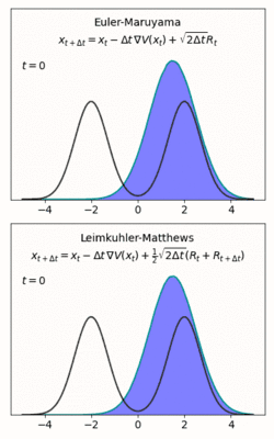
Leimkuhler–Matthews method

In mathematics, the Leimkuhler-Matthews method (or LM method in its original paper ) is an algorithm for finding discretized solutions to the Brownian dynamics

[math]\displaystyle{ \mathrm{d} X = -\nabla V(X ) \, \mathrm{d} t + \sigma \, \mathrm{d} W, }[/math]

where [math]\displaystyle{ \sigma\gt 0 }[/math] is a constant, [math]\displaystyle{ V(X) }[/math] is an energy function and [math]\displaystyle{ W(t) }[/math] is a Wiener process. This stochastic differential equation has solutions (denoted [math]\displaystyle{ X(t) \in \mathbb{R}^N }[/math] at time [math]\displaystyle{ t }[/math]) distributed according to [math]\displaystyle{ \pi(X) \propto \exp(-V(x)) }[/math] in the limit of large-time, making solving these dynamics relevant in sampling-focused applications such as classical molecular dynamics and machine learning.

Given a time step [math]\displaystyle{ \Delta t\gt 0 }[/math], the Leimkuhler-Matthews update scheme is compactly written as

[math]\displaystyle{ X_{t+\Delta t} = X_t -\nabla V(X_t) \Delta t + \sigma\frac{\sqrt{\Delta t}}2 \, (R_t+R_{t+\Delta t}), }[/math]

with initial condition [math]\displaystyle{ X_0 := X(0) }[/math], and where [math]\displaystyle{ X_t \approx X(t) }[/math]. The vector [math]\displaystyle{ R_t }[/math] is a vector of independent normal random numbers redrawn at each step so [math]\displaystyle{ \text{E}[ R_t \cdot R_{s}]=N\delta_{ts} }[/math] (where [math]\displaystyle{ \text{E}[\bullet] }[/math] denotes expectation). Despite being of equal cost to the Euler-Maruyama scheme (in terms of the number of evaluations of the function [math]\displaystyle{ \nabla V(X) }[/math] per update), given some assumptions on [math]\displaystyle{ \Delta t,\, V(X) }[/math] and [math]\displaystyle{ f(X) }[/math] solutions have been shown to have a superconvergence property

[math]\displaystyle{ \text{E}[|f( X_t ) - f(X(t))|] \leq C_1 e^{-\lambda t} \Delta t + C_2 \Delta t^2 }[/math]

for constants [math]\displaystyle{ C_k\geq0,\, \lambda\gt 0 }[/math] not depending on [math]\displaystyle{ t }[/math]. This means that as [math]\displaystyle{ t }[/math] gets large we obtain an effective second order with [math]\displaystyle{ \Delta t^2 }[/math] error in computed expectations. For small time step [math]\displaystyle{ \Delta t }[/math] this can give significant improvements over the Euler-Maruyama scheme, at no extra cost.

Discussion

The distribution of solutions at time [math]\displaystyle{ t }[/math] for the Euler-Maruyama method and the Leimkuhler-Matthews method, using discretization [math]\displaystyle{ \Delta t=0.5 }[/math] and initializing from a Normal distribution. The target distribution (in black) is the sum of two Gaussian distributions centered at [math]\displaystyle{ -2 }[/math] and [math]\displaystyle{ +2 }[/math]. While the Euler-Maruyama scheme results in a visible discretization error in the sampled distribution, the Leimkuhler-Matthews scheme performs significantly better for no extra cost.

Comparison to other schemes

The obvious method for comparison is the Euler-Maruyama scheme as it has the same cost, requiring one evaluation of [math]\displaystyle{ \nabla V(X) }[/math] per step. Its update is of the form

[math]\displaystyle{ \hat{X}_{t+\Delta t} = \hat{X}_t -\nabla V(\hat{X}_t) \Delta t + \sigma{\sqrt{\Delta t}} \, R_t, }[/math]

with error (given some assumptions ) as [math]\displaystyle{ \text{E}[|f(\hat{X}_{t}) - f(X(t))|] \leq C \Delta t }[/math] with constant [math]\displaystyle{ C\gt 0 }[/math] independent of [math]\displaystyle{ t }[/math]. Compared to the above definition, the only difference between the schemes is the one-step averaged noise term, making it simple to implement.

For sufficiently small time step [math]\displaystyle{ \Delta t }[/math] and large enough time [math]\displaystyle{ t }[/math] it is clear that the LM scheme gives a smaller error than Euler-Maruyama. While there are many algorithms that can give reduced error compared to the Euler scheme (see e.g. Milstein, Runge-Kutta or Heun's method) these almost always come at an efficiency cost, requiring more computation in exchange for reducing the error. However the Leimkuhler-Matthews scheme can give significantly reduced error with minimal change to the standard Euler scheme. The trade-off comes from the (relatively) limited scope of the stochastic differential equation it solves: [math]\displaystyle{ \sigma }[/math] must be a scalar constant and the drift function must be of the form [math]\displaystyle{ \nabla V(X) }[/math]. The LM scheme also is not Markovian, as updates require more than just the state at time [math]\displaystyle{ t }[/math]. However, we can recast the scheme as a Markov process by extending the space.

Markovian Form

We can rewrite the algorithm in a Markovian form by extending the state space with a momentum vector [math]\displaystyle{ P_t\in\mathbb{R}^N }[/math] so that the overall state is [math]\displaystyle{ (X_t,P_t) }[/math] at time [math]\displaystyle{ t }[/math]. Initializing the momentum to be a vector of [math]\displaystyle{ N }[/math] standard normal random numbers, we have

[math]\displaystyle{ X'_{t+\Delta t} = X_t -\nabla V(X_t) \Delta t + \sigma\frac{\sqrt{\Delta t}}2 \, P_t, }[/math]

[math]\displaystyle{ P_{t+\Delta t} \sim \text{Normal}(0,I), }[/math]

[math]\displaystyle{ X_{t+\Delta t} = X'_{t+\Delta t} + \sigma\frac{\sqrt{\Delta t}}2 \, P_{t+\Delta t}, }[/math]

where the middle step completely redraws the momentum so that each component is an independent normal random number. This scheme is Markovian, and has the same properties as the original LM scheme.

Applications

The algorithm has application in any area where the weak (i.e. average) properties of solutions to Brownian dynamics are required. This applies to any molecular simulation problem (such as classical molecular dynamics), but also can apply to statistical sampling problems due to the properties of solutions at large times. In the limit of [math]\displaystyle{ t\to\infty }[/math], solutions will become distributed according to the Probability distribution [math]\displaystyle{ \pi(X) \propto \exp(-V(X)) }[/math]. Thus we can generate independent samples according to a required distribution by using [math]\displaystyle{ V(X) = -\log(\pi(X)) }[/math] and running the LM algorithm until large [math]\displaystyle{ t }[/math]. Such strategies can be efficient in (for instance) Bayesian inference problems.

See also

• Euler-Maruyama method
• Milstein method
• Runge–Kutta method (SDE)
• Heun's method

References

- ↑ Leimkuhler, Benedict; Matthews, Charles (1 January 2013). "Rational Construction of Stochastic Numerical Methods for Molecular Sampling" (in en). Applied Mathematics Research EXpress 2013 (1): 34–56. doi:10.1093/amrx/abs010. ISSN 1687-1200. https://academic.oup.com/amrx/article/2013/1/34/166771.
- ↑ Leimkuhler, B.; Matthews, C.; Tretyakov, M. V. (8 October 2014). "On the long-time integration of stochastic gradient systems". Proceedings of the Royal Society A: Mathematical, Physical and Engineering Sciences 470 (2170): 20140120. doi:10.1098/rspa.2014.0120. Bibcode: 2014RSPSA.47040120L.
- ↑ Kloeden, P.E.; Platen, E. (1992). Numerical Solution of Stochastic Differential Equations. Springer, Berlin. ISBN 3-540-54062-8.