Log-Cauchy distribution
|
Probability density function  | |||
|
Cumulative distribution function  | |||
| Parameters |
(real) (real) | ||
|---|---|---|---|
| Support | |||
| CDF | |||
| Mean | infinite | ||
| Median | |||
| Variance | infinite | ||
| Skewness | does not exist | ||
| Kurtosis | does not exist | ||
| MGF | does not exist | ||
In probability theory, a log-Cauchy distribution is a probability distribution of a random variable whose logarithm is distributed in accordance with a Cauchy distribution. If X is a random variable with a Cauchy distribution, then Y = exp(X) has a log-Cauchy distribution; likewise, if Y has a log-Cauchy distribution, then X = log(Y) has a Cauchy distribution.[1]
Characterization
The log-Cauchy distribution is a special case of the log-t distribution where the degrees of freedom parameter is equal to 1.[2]
Probability density function
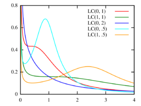
The log-Cauchy distribution has the probability density function:
where is a real number and .[1][3] If is known, the scale parameter is .[1] and correspond to the location parameter and scale parameter of the associated Cauchy distribution.[1][4] Some authors define and as the location and scale parameters, respectively, of the log-Cauchy distribution.[4]
For and , corresponding to a standard Cauchy distribution, the probability density function reduces to:[5]
Cumulative distribution function
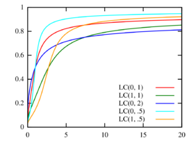
The cumulative distribution function (cdf) when and is:[5]
Survival function
The survival function when and is:[5]
Hazard rate
The hazard rate when and is:[5]
The hazard rate decreases at the beginning and at the end of the distribution, but there may be an interval over which the hazard rate increases.[5]
Properties
The log-Cauchy distribution is an example of a heavy-tailed distribution.[6] Some authors regard it as a "super-heavy tailed" distribution, because it has a heavier tail than a Pareto distribution-type heavy tail, i.e., it has a logarithmically decaying tail.[6][7] As with the Cauchy distribution, none of the non-trivial moments of the log-Cauchy distribution are finite.[5] The mean is a moment so the log-Cauchy distribution does not have a defined mean or standard deviation.[8][9]
The log-Cauchy distribution is infinitely divisible for some parameters but not for others.[10] Like the lognormal distribution, log-t or log-Student distribution and Weibull distribution, the log-Cauchy distribution is a special case of the generalized beta distribution of the second kind.[11][12] The log-Cauchy is actually a special case of the log-t distribution, similar to the Cauchy distribution being a special case of the Student's t distribution with 1 degree of freedom.[13][14]
Since the Cauchy distribution is a stable distribution, the log-Cauchy distribution is a logstable distribution.[15] Logstable distributions have poles at x=0.[14]
Estimating parameters
The median of the natural logarithms of a sample is a robust estimator of .[1] The median absolute deviation of the natural logarithms of a sample is a robust estimator of .[1]
Uses
In Bayesian statistics, the log-Cauchy distribution can be used to approximate the improper Jeffreys-Haldane density, 1/k, which is sometimes suggested as the prior distribution for k where k is a positive parameter being estimated.[16][17] The log-Cauchy distribution can be used to model certain survival processes where significant outliers or extreme results may occur.[3][4][18] An example of a process where a log-Cauchy distribution may be an appropriate model is the time between someone becoming infected with HIV and showing symptoms of the disease, which may be very long for some people.[4] It has also been proposed as a model for species abundance patterns.[19]
References
- ↑ 1.0 1.1 1.2 1.3 1.4 1.5 Olive, D.J. (June 23, 2008). "Applied Robust Statistics". Southern Illinois University. p. 86. http://www.math.siu.edu/olive/run.pdf.
- ↑ Olosunde, Akinlolu & Olofintuade, Sylvester (January 2022). "Some Inferential Problems from Log Student's T-distribution and its Multivariate Extension". Revista Colombiana de Estadística - Applied Statistics 45 (1): 209–229. doi:10.15446/rce.v45n1.90672. https://www.proquest.com/openview/70d41b2007ad2f9ade89ed9ef6eba775/1?pq-origsite=gscholar&cbl=2035762. Retrieved 2022-04-01.
- ↑ 3.0 3.1 Lindsey, J.K. (2004). Statistical analysis of stochastic processes in time. Cambridge University Press. pp. 33, 50, 56, 62, 145. ISBN 978-0-521-83741-5. https://archive.org/details/statisticalanaly00lind.
- ↑ 4.0 4.1 4.2 4.3 Mode, C.J.; Sleeman, C.K. (2000). Stochastic processes in epidemiology: HIV/AIDS, other infectious diseases. World Scientific. pp. 29–37. ISBN 978-981-02-4097-4. https://archive.org/details/stochasticproces00mode.
- ↑ 5.0 5.1 5.2 5.3 5.4 5.5 Marshall, A.W.; Olkin, I. (2007). Life distributions: structure of nonparametric, semiparametric, and parametric families. Springer. pp. 443–444. ISBN 978-0-387-20333-1. https://archive.org/details/lifedistribution00mars.
- ↑ 6.0 6.1 Falk, M.; Hüsler, J.; Reiss, R. (2010). Laws of Small Numbers: Extremes and Rare Events. Springer. p. 80. ISBN 978-3-0348-0008-2. https://archive.org/details/lawssmallnumbers00falk.
- ↑ Alves, M.I.F.; de Haan, L. (March 10, 2006). "Statistical inference for heavy and super-heavy tailed distributions". http://docentes.deio.fc.ul.pt/fragaalves/SuperHeavy.pdf.
- ↑ "Moment". Mathworld. http://mathworld.wolfram.com/Moment.html.
- ↑ Wang, Y.. Trade, Human Capital and Technology Spillovers: An Industry Level Analysis. Carleton University. p. 14.
- ↑ Bondesson, L. (2003). "On the Lévy Measure of the Lognormal and LogCauchy Distributions". Methodology and Computing in Applied Probability: 243–256. http://resources.metapress.com/pdf-preview.axd?code=gn16hw202rxh4q1g&size=largest. Retrieved 2011-10-18.
- ↑ Knight, J.; Satchell, S. (2001). Return distributions in finance. Butterworth-Heinemann. p. 153. ISBN 978-0-7506-4751-9. https://archive.org/details/returndistributi00satc_172.
- ↑ Kemp, M. (2009). Market consistency: model calibration in imperfect markets. Wiley. ISBN 978-0-470-77088-7.
- ↑ MacDonald, J.B. (1981). "Measuring Income Inequality". in Taillie, C.. Statistical distributions in scientific work: proceedings of the NATO Advanced Study Institute. Springer. p. 169. ISBN 978-90-277-1334-6.
- ↑ 14.0 14.1 Kleiber, C.; Kotz, S. (2003). Statistical Size Distributions in Economics and Actuarial Science. Wiley. pp. 101–102, 110. ISBN 978-0-471-15064-0. https://archive.org/details/statisticalsized0000unse.
- ↑ Panton, D.B. (May 1993). "Distribution function values for logstable distributions". Computers & Mathematics with Applications 25 (9): 17–24. doi:10.1016/0898-1221(93)90128-I.
- ↑ Good, I.J. (1983). Good thinking: the foundations of probability and its applications. University of Minnesota Press. p. 102. ISBN 978-0-8166-1142-3.
- ↑ Chen, M. (2010). Frontiers of Statistical Decision Making and Bayesian Analysis. Springer. p. 12. ISBN 978-1-4419-6943-9.
- ↑ Lindsey, J.K.; Jones, B.; Jarvis, P. (September 2001). "Some statistical issues in modelling pharmacokinetic data". Statistics in Medicine 20 (17–18): 2775–278. doi:10.1002/sim.742. PMID 11523082.
- ↑ Zuo-Yun, Y. (June 2005). "LogCauchy, log-sech and lognormal distributions of species abundances in forest communities". Ecological Modelling 184 (2–4): 329–340. doi:10.1016/j.ecolmodel.2004.10.011. Bibcode: 2005EcMod.184..329Y.
 |
