Generalized beta distribution

In probability and statistics, the generalized beta distribution is a continuous probability distribution with four shape parameters (however it's customary to make explicit the scale parameter as a fifth parameter, while the location parameter is usually left implicit), including more than thirty named distributions as limiting or special cases. It has been used in the modeling of income distribution, stock returns, as well as in regression analysis. The exponential generalized beta (EGB) distribution follows directly from the GB and generalizes other common distributions.

Definition

A generalized beta random variable, Y, is defined by the following probability density function:

[math]\displaystyle{ GB(y;a,b,c,p,q) = \frac{|a|y^{ap-1}(1-(1-c)(y/b)^{a})^{q-1}}{b^{ap}B(p,q)(1+c(y/b)^{a})^{p+q}} \quad \quad \text{ for } 0\lt y^{a}\lt \frac{b^a}{1-c} , }[/math]

and zero otherwise. Here the parameters satisfy [math]\displaystyle{ a \ne 0 }[/math], [math]\displaystyle{ 0 \le c \le 1 }[/math] and [math]\displaystyle{ b }[/math], [math]\displaystyle{ p }[/math], and [math]\displaystyle{ q }[/math] positive. The function B(p,q) is the beta function. The parameter [math]\displaystyle{ b }[/math] is the scale parameter and can thus be set to [math]\displaystyle{ 1 }[/math] without loss of generality, but it is usually made explicit as in the function above (while the location parameter is usually left implicit and set to [math]\displaystyle{ 0 }[/math] as in the function above).

GB distribution tree

Properties

Moments

It can be shown that the hth moment can be expressed as follows:

[math]\displaystyle{ \operatorname{E}_{GB}(Y^{h})=\frac{b^{h}B(p+h/a,q)}{B(p,q)}{}_{2}F_{1} \begin{bmatrix} p + h/a,h/a;c \\ p + q +h/a; \end{bmatrix}, }[/math]

where [math]\displaystyle{ {}_{2}F_{1} }[/math] denotes the hypergeometric series (which converges for all h if c<1, or for all h/a<q if c=1 ).

Related distributions

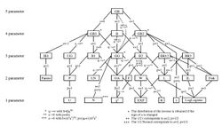
The generalized beta encompasses many distributions as limiting or special cases. These are depicted in the GB distribution tree shown above. Listed below are its three direct descendants, or sub-families.

Generalized beta of first kind (GB1)

The generalized beta of the first kind is defined by the following pdf:

[math]\displaystyle{ GB1(y;a,b,p,q) = \frac{|a|y^{ap-1}(1-(y/b)^{a})^{q-1}}{b^{ap}B(p,q)} }[/math]

for [math]\displaystyle{ 0\lt y^{a}\lt b^{a} }[/math] where [math]\displaystyle{ b }[/math], [math]\displaystyle{ p }[/math], and [math]\displaystyle{ q }[/math] are positive. It is easily verified that

[math]\displaystyle{ GB1(y;a,b,p,q) = GB(y;a,b,c=0,p,q). }[/math]

The moments of the GB1 are given by

[math]\displaystyle{ \operatorname{E}_{GB1}(Y^{h}) = \frac{b^{h}B(p+h/a,q)}{B(p,q)}. }[/math]

The GB1 includes the beta of the first kind (B1), generalized gamma(GG), and Pareto as special cases:

[math]\displaystyle{ B1(y;b,p,q) = GB1(y;a=1,b,p,q) , }[/math]

[math]\displaystyle{ GG(y;a,\beta,p) = \lim_{q \to \infty} GB1(y;a,b=q^{1/a}\beta,p,q) , }[/math]

[math]\displaystyle{ PARETO(y;b,p) = GB1(y;a=-1,b,p,q=1) . }[/math]

Generalized beta of the second kind (GB2)

The GB2 is defined by the following pdf:

[math]\displaystyle{ GB2(y;a,b,p,q) = \frac{|a|y^{ap-1}}{b^{ap}B(p,q)(1+(y/b)^a)^{p+q}} }[/math]

for [math]\displaystyle{ 0\lt y \lt \infty }[/math] and zero otherwise. One can verify that

[math]\displaystyle{ GB2(y;a,b,p,q) = GB(y;a,b,c=1,p,q). }[/math]

The moments of the GB2 are given by

[math]\displaystyle{ \operatorname{E}_{GB2}(Y^h) = \frac{b^h B(p+h/a,q-h/a)}{B(p,q)}. }[/math]

The GB2 is also known as the Generalized Beta Prime (Patil, Boswell, Ratnaparkhi (1984)), the transformed beta (Venter, 1983), the generalized F (Kalfleisch and Prentice, 1980), and is a special case (μ≡0) of the Feller-Pareto (Arnold, 1983) distribution. The GB2 nests common distributions such as the generalized gamma (GG), Burr type 3, Burr type 12, Dagum, lognormal, Weibull, gamma, Lomax, F statistic, Fisk or Rayleigh, chi-square, half-normal, half-Student's t, exponential, asymmetric log-Laplace, log-Laplace, power function, and the log-logistic.

Beta

The beta family of distributions (B) is defined by:

[math]\displaystyle{ B(y;b,c,p,q) = \frac{y^{p-1}(1-(1-c)(y/b))^{q-1}}{b^{p}B(p,q)(1+c(y/b))^{p+q}} }[/math]

for [math]\displaystyle{ 0\lt y\lt b/(1-c) }[/math] and zero otherwise. Its relation to the GB is seen below:

[math]\displaystyle{ B(y;b,c,p,q) = GB(y;a=1,b,c,p,q). }[/math]

The beta family includes the beta of the first and second kind (B1 and B2, where the B2 is also referred to as the Beta prime), which correspond to c = 0 and c = 1, respectively. Setting [math]\displaystyle{ c = 0 }[/math], [math]\displaystyle{ b = 1 }[/math] yields the standard two-parameter beta distribution.

Generalized Gamma

The generalized gamma distribution (GG) is a limiting case of the GB2. Its PDF is defined by:

[math]\displaystyle{ GG(y;a,\beta,p) = \lim_{q \rightarrow \infty} GB2(y,a,b=q^{1/a} \beta,p,q) = \frac{|a|y^{ap-1}e^{-(y/\beta)^{a}}}{\beta^{ap} \Gamma (p)} }[/math]

with the [math]\displaystyle{ h }[/math]th moments given by

[math]\displaystyle{ \operatorname{E}(Y_{GG}^h) = \frac{\beta^h \Gamma (p + h/a)}{\Gamma (p)}. }[/math]

As noted earlier, the GB distribution family tree visually depicts the special and limiting cases (see McDonald and Xu (1995) ).

Pareto

The Pareto (PA) distribution is the following limiting case of the generalized gamma:

[math]\displaystyle{ PA(y;\beta,\theta) = \lim_{a \rightarrow -\infty} GG(y;a,\beta,p=-\theta /a) = \lim_{a \rightarrow -\infty}\left(\frac{\theta y^{-\theta-1}e^{-(y/\beta)^{a}}}{\beta^{-\theta}(-\theta / a)\Gamma(-\theta / a)}\right) = }[/math]

[math]\displaystyle{ \lim_{a \rightarrow -\infty}\left(\frac{\theta y^{-\theta - 1}e^{-(y/\beta)^{a}}}{\beta^{-\theta}\Gamma(1-\theta / a)} \right) = \frac{\theta y^{-\theta - 1}}{\beta^{-\theta}} }[/math] for [math]\displaystyle{ \beta \lt y }[/math] and [math]\displaystyle{ 0 }[/math] otherwise.

Power

The power (P) distribution is the following limiting case of the generalized gamma:

[math]\displaystyle{ P(y;\beta,\theta) = \lim_{a\rightarrow\infty}GG(y;a=\theta /p, \beta, p) = \lim_{a\rightarrow\infty}\frac{\mid\frac{\theta}{p}|y^{\theta-1}e^{-(y/\beta)^a}}{\beta^{\theta}\Gamma(p)} = \lim_{a\rightarrow\infty}\frac{\theta y^{\theta - 1}}{p\Gamma(p)\beta^{\theta}}e^{-(y/\beta)^{a}} = }[/math]

[math]\displaystyle{ \lim_{a\rightarrow\infty}\frac{\theta y^{\theta - 1}}{\Gamma(p + 1)\beta^{\theta}}e^{-(y/\beta)^{a}} = \lim_{a\rightarrow\infty}\frac{\theta y^{\theta - 1}}{\Gamma(\frac{\theta}{a} + 1)\beta^{\theta}}e^{-(y/\beta)^{a}} = \frac{\theta y^{\theta - 1}}{\beta^{\theta}}, }[/math]

which is equivalent to the power function distribution for [math]\displaystyle{ 0\leq y\leq\beta }[/math] and [math]\displaystyle{ \theta \gt 0 }[/math].

Asymmetric Log-Laplace

The asymmetric log-Laplace distribution (also referred to as the double Pareto distribution ) is defined by:

[math]\displaystyle{ ALL(y;b,\lambda_1,\lambda_2) = \lim_{a \rightarrow \infty} GB2(y;a,b,p = \lambda_1/a,q = \lambda_2/a) = \frac{\lambda_1\lambda_2}{y(\lambda_1+\lambda_2)}\begin{cases} (\frac{y}{b})^{\lambda_1} & \mbox{for } 0 \lt y \lt b \\ (\frac{b}{y})^{\lambda_2} & \mbox{for } y \ge b \end{cases} }[/math]

where the [math]\displaystyle{ h }[/math]th moments are given by

[math]\displaystyle{ \operatorname{E}(Y_{ALL}^h) = \frac{b^h \lambda_1 \lambda_2}{(\lambda_1 + h)(\lambda_2 - h)}. }[/math]

When [math]\displaystyle{ \lambda_1 = \lambda_2 }[/math], this is equivalent to the log-Laplace distribution.

Exponential generalized beta distribution

Letting [math]\displaystyle{ Y \sim GB(y;a,b,c,p,q) }[/math] (without location parameter), the random variable [math]\displaystyle{ Z = \ln(Y) }[/math], with re-parametrization [math]\displaystyle{ \delta = \ln(b) }[/math] and [math]\displaystyle{ \sigma = 1/a }[/math], is distributed as an exponential generalized beta (EGB), with the following pdf:

[math]\displaystyle{ EGB(z;\delta,\sigma,c,p,q) = \frac{e^{p(z-\delta)/\sigma}(1-(1-c)e^{(z-\delta)/\sigma})^{q-1}}{|\sigma|B(p,q)(1+ce^{(z-\delta)/\sigma})^{p+q}} }[/math]

for [math]\displaystyle{ -\infty \lt \frac{z-\delta}{\sigma}\lt \ln(\frac{1}{1-c}) }[/math], and zero otherwise. The EGB includes generalizations of the Gompertz, Gumbel, extreme value type I, logistic, Burr-2, exponential, and normal distributions. The parameter [math]\displaystyle{ \delta = \ln(b) }[/math] is the location parameter of the EGB (while [math]\displaystyle{ b }[/math] is the scale parameter of the GB), and [math]\displaystyle{ \sigma = 1/a }[/math] is the scale parameter of the EGB (while [math]\displaystyle{ a }[/math] is a shape parameter of the GB); The EGB has thus three shape parameters.

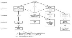
Included is a figure showing the relationship between the EGB and its special and limiting cases.

The EGB family of distributions

Moment generating function

Using similar notation as above, the moment-generating function of the EGB can be expressed as follows:

[math]\displaystyle{ M_{EGB}(Z)=\frac{e^{\delta t}B(p+t\sigma,q)}{B(p,q)}{}_{2}F_{1} \begin{bmatrix} p + t\sigma,t\sigma;c \\ p + q +t\sigma; \end{bmatrix}. }[/math]

Multivariate generalized beta distribution

A multivariate generalized beta pdf extends the univariate distributions listed above. For [math]\displaystyle{ n }[/math] variables [math]\displaystyle{ y = (y_1 , ... , y_n) }[/math], define [math]\displaystyle{ 1xn }[/math] parameter vectors by [math]\displaystyle{ a = (a_1 , ... , a_n) }[/math], [math]\displaystyle{ b = (b_1 , ... , b_n) }[/math], [math]\displaystyle{ c = (c_1 , ... , c_n) }[/math], and [math]\displaystyle{ p = (p_1 , ... , p_n) }[/math] where each [math]\displaystyle{ b_i }[/math] and [math]\displaystyle{ p_i }[/math] is positive, and [math]\displaystyle{ 0 }[/math] [math]\displaystyle{ \le }[/math] [math]\displaystyle{ c_i }[/math] [math]\displaystyle{ \le }[/math] [math]\displaystyle{ 1 }[/math]. The parameter [math]\displaystyle{ q }[/math] is assumed to be positive, and define the function [math]\displaystyle{ B(p_1, ... , p_n, q) }[/math] = [math]\displaystyle{ \frac{\Gamma(p_1)...\Gamma(p_n)\Gamma(q)}{\Gamma(\bar{p}+q)} }[/math] for [math]\displaystyle{ \bar{p} }[/math] = [math]\displaystyle{ \sum_{i=1}^{n} p_i }[/math].

The pdf of the multivariate generalized beta ([math]\displaystyle{ MGB }[/math]) may be written as follows:

[math]\displaystyle{ MGB(y; a, b, p, q, c) = \frac{(\prod_{i=1}^{n} |a_i|y_i^{a_i p_i - 1})(1 - \sum_{i=1}^{n} (1-c_i)(\frac{y_i}{b_i})^{a_i})^{q - 1}}{(\prod_{i=1}^{n} b_i^{a_i p_i})B(p_1, ... , p_n, q)(1 + \sum_{i=1}^{n} c_i(\frac{y_i}{b_i})^{a_i})^{\bar{p} + q}} }[/math]

where [math]\displaystyle{ 0 }[/math] [math]\displaystyle{ \lt }[/math] [math]\displaystyle{ \sum_{i=1}^{n} (1-c_i)(\frac{y_i}{b_i})^{a_i} }[/math] [math]\displaystyle{ \lt }[/math] [math]\displaystyle{ 1 }[/math] for [math]\displaystyle{ 0 }[/math] [math]\displaystyle{ \le }[/math] [math]\displaystyle{ c_i }[/math] [math]\displaystyle{ \lt }[/math] [math]\displaystyle{ 1 }[/math] and [math]\displaystyle{ 0 }[/math] [math]\displaystyle{ \lt }[/math] [math]\displaystyle{ y_i }[/math] when [math]\displaystyle{ c_i }[/math] = [math]\displaystyle{ 1 }[/math].

Like the univariate generalized beta distribution, the multivariate generalized beta includes several distributions in its family as special cases. By imposing certain constraints on the parameter vectors, the following distributions can be easily derived.

Multivariate generalized beta of the first kind (MGB1)

When each [math]\displaystyle{ c_i }[/math] is equal to 0, the MGB function simplifies to the multivariate generalized beta of the first kind (MGB1), which is defined by:

[math]\displaystyle{ MGB1(y; a, b, p, q) = \frac{(\prod_{i=1}^{n} |a_i|y_i^{a_i p_i - 1})(1 - \sum_{i=1}^{n} (\frac{y_i}{b_i})^{a_i})^{q - 1}}{(\prod_{i=1}^{n} b_i^{a_i p_i})B(p_1, ... , p_n, q)} }[/math]

where [math]\displaystyle{ 0 }[/math] [math]\displaystyle{ \lt }[/math] [math]\displaystyle{ \sum_{i=1}^{n} (\frac{y_i}{b_i})^{a_i} }[/math] [math]\displaystyle{ \lt }[/math] [math]\displaystyle{ 1 }[/math].

Multivariate generalized beta of the second kind (MGB2)

In the case where each [math]\displaystyle{ c_i }[/math] is equal to 1, the MGB simplifies to the multivariate generalized beta of the second kind (MGB2), with the pdf defined below:

[math]\displaystyle{ MGB2(y; a, b, p, q) = \frac{(\prod_{i=1}^{n} |a_i|y_i^{a_i p_i - 1})}{(\prod_{i=1}^{n} b_i^{a_i p_i})B(p_1, ... , p_n, q)(1 + \sum_{i=1}^{n} (\frac{y_i}{b_i})^{a_i})^{\bar{p} + q}} }[/math]

when [math]\displaystyle{ 0 }[/math] [math]\displaystyle{ \lt }[/math] [math]\displaystyle{ y_i }[/math] for all [math]\displaystyle{ y_i }[/math].

Multivariate generalized gamma

The multivariate generalized gamma (MGG) pdf can be derived from the MGB pdf by substituting [math]\displaystyle{ b_i }[/math] = [math]\displaystyle{ \beta_i q ^ {\frac{1}{a_i}} }[/math] and taking the limit as [math]\displaystyle{ q }[/math] [math]\displaystyle{ \to }[/math] [math]\displaystyle{ \infty }[/math], with Stirling's approximation for the gamma function, yielding the following function:

[math]\displaystyle{ MGG(y; a, \beta, p) = (\frac{(\prod_{i=1}^{n} |a_i|y_i^{a_i p_i - 1})}{(\prod_{i=1}^{n} \beta_i^{a_i p_i})\Gamma(p_i)})e^{- \sum_{i=1}^{n} (\frac{y_i}{\beta_i})^{a_i}} = \prod_{i=1}^{n} GG(y_i; a_i, \beta_i, p_i) }[/math]

which is the product of independently but not necessarily identically distributed generalized gamma random variables.

Other multivariate distributions

Similar pdfs can be constructed for other variables in the family tree shown above, simply by placing an M in front of each pdf name and finding the appropriate limiting and special cases of the MGB as indicated by the constraints and limits of the univariate distribution. Additional multivariate pdfs in the literature include the Dirichlet distribution (standard form) given by [math]\displaystyle{ MGB1(y; a = 1, b = 1, p, q) }[/math], the multivariate inverted beta and inverted Dirichlet (Dirichlet type 2) distribution given by [math]\displaystyle{ MGB2(y; a = 1, b = 1, p, q) }[/math], and the multivariate Burr distribution given by [math]\displaystyle{ MGB2(y; a, b, p, q = 1) }[/math].

Marginal density functions

The marginal density functions of the MGB1 and MGB2, respectively, are the generalized beta distributions of the first and second kind, and are given as follows:

[math]\displaystyle{ GB1(y_i; a_i, b_i, p_i, \bar{p} - p_i + q) = \frac{|a_i|y_i^{a_i p_i - 1}(1 - (\frac{y_i}{b_i})^{a_i})^{\bar{p} - p_i + q - 1}}{b_i^{a_i p_i}B(p_i, \bar{p} - p_i + q)} }[/math]

[math]\displaystyle{ GB2(y_i; a_i, b_i, p_i, q) = \frac{|a_i|y_i^{a_i p_i - 1}}{b_i^{a_i p_i}B(p_i, q)(1 + (\frac{y_i}{b_i})^{a_i})^{p_i + q}} }[/math]

Applications

The flexibility provided by the GB family is used in modeling the distribution of:

• distribution of income
• hazard functions
• stock returns
• insurance losses

Applications involving members of the EGB family include:

• partially adaptive estimation of regression models
• time series models
• (G)ARCH models

Distribution of Income

The GB2 and several of its special and limiting cases have been widely used as models for the distribution of income. For some early examples see Thurow (1970), Dagum (1977), Singh and Maddala (1976), and McDonald (1984). Maximum likelihood estimations using individual, grouped, or top-coded data are easily performed with these distributions.

Measures of inequality, such as the Gini index (G), Pietra index (P), and Theil index (T) can be expressed in terms of the distributional parameters, as given by McDonald and Ransom (2008):

[math]\displaystyle{ \begin{align} G=\left({\frac{1}{2\mu}}\right) \operatorname{E}(|Y-X|) = \left(P{\frac{1}{2\mu}}\right) \int_{0}^{\infty}\int_{0}^{\infty} |x-y|f(x)f(y)\,dx dy \\ = 1 - \frac{\int_{0}^{\infty} (1-F(y))^2\,dy}{\int_{0}^{\infty} (1-F(y))\,dy} \\ P = \left( \frac{1}{2\mu}\right) \operatorname{E} (|Y-\mu|) = \left(\frac{1}{2\mu}\right)\int_0^{\infty} |y-\mu|f(y)\, dy \\ T = \operatorname{E} (\ln (Y/\mu)^{Y/\mu}) = \int_0^ \infty (y/\mu) \ln (y/\mu) f(y)\, dy \end{align} }[/math]

Hazard Functions

The hazard function, h(s), where f(s) is a pdf and F(s) the corresponding cdf, is defined by

[math]\displaystyle{ h(s) = \frac{f(s)}{1-F(s)} }[/math]

Hazard functions are useful in many applications, such as modeling unemployment duration, the failure time of products or life expectancy. Taking a specific example, if s denotes the length of life, then h(s) is the rate of death at age s, given that an individual has lived up to age s. The shape of the hazard function for human mortality data might appear as follows: decreasing mortality in the first few months of life, then a period of relatively constant mortality and finally an increasing probability of death at older ages.

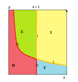
Special cases of the generalized beta distribution offer more flexibility in modeling the shape of the hazard function, which can call for "∪" or "∩" shapes or strictly increasing (denoted by I}) or decreasing (denoted by D) lines. The generalized gamma is "∪"-shaped for a>1 and p<1/a, "∩"-shaped for a<1 and p>1/a, I-shaped for a>1 and p>1/a and D-shaped for a<1 and p>1/a. This is summarized in the figure below.

Possible hazard function shapes using the generalized gamma

Bibliography

• C. Kleiber and S. Kotz (2003) Statistical Size Distributions in Economics and Actuarial Sciences. New York: Wiley
• Johnson, N. L., S. Kotz, and N. Balakrishnan (1994) Continuous Univariate Distributions. Vol. 2, Hoboken, NJ: Wiley-Interscience.

References

- ↑ 1.0 1.1 1.2 McDonald, James B. & Xu, Yexiao J. (1995) "A generalization of the beta distribution with applications," Journal of Econometrics, 66(1–2), 133–152 doi:10.1016/0304-4076(94)01612-4
- ↑ Patil, G.P., Boswell, M.T., and Ratnaparkhi, M.V., Dictionary and Classified Bibliography of Statistical Distributions in Scientific Work Series, editor G.P. Patil, Internal Co-operative Publishing House, Burtonsville, Maryland, 1984.
- ↑ Venter, G., Transformed beta and gamma distributions and aggregate losses, Proceedings of the Casualty Actuarial Society, 1983.
- ↑ Kalbfleisch, J.D. and R.L. Prentice, The Statistical Analysis of Failure Time Data, New York: J. Wiley, 1980
- ↑ Arnold, B.C., Pareto Distributions, Volume 5 in Statistical Distributions in Scientific Work Series, International Co-operative Publishing House, Burtonsville, Md. 1983.
- ↑ 6.0 6.1 6.2 McDonald, J.B. (1984) "Some generalized functions for the size distributions of income", Econometrica 52, 647–663.
- ↑ Stuart, A. and Ord, J.K. (1987): Kendall's Advanced Theory of Statistics, New York: Oxford University Press.
- ↑ Stacy, E.W. (1962). "A Generalization of the Gamma Distribution." Annals of Mathematical Statistics 33(3): 1187-1192. JSTOR 2237889
- ↑ Reed, W.J. (2001). "The Pareto, Zipf, and other power laws." Economics Letters 74: 15-19. doi:10.1016/S0165-1765(01)00524-9
- ↑ Higbee, J.D., Jensen, J.E., and McDonald, J.B. (2019). "The asymmetric log-Laplace distribution as a limiting case of the generalized beta distribution."Statistics and Probability Letters 151: 73-78. doi:10.1016/j.spl.2019.03.018
- ↑ McDonald, James B. & Kerman, Sean C. (2013) "Skewness-Kurtosis Bounds for EGB1, EGB2, and Special Cases," Forthcoming
- ↑ William M. Cockriel & James B. McDonald (2017): Two multivariate generalized beta families, Communications in Statistics - Theory and Methods, doi:10.1080/03610926.2017.1400058
- ↑ Thurow, L.C. (1970) "Analyzing the American Income Distribution," Papers and Proceedings, American Economics Association, 60, 261-269
- ↑ Dagum, C. (1977) "A New Model for Personal Income Distribution: Specification and Estimation," Economie Applique'e, 30, 413-437
- ↑ Singh, S.K. and Maddala, G.S (1976) "A Function for the Size Distribution of Incomes," Econometrica, 44, 963-970
- ↑ McDonald, J.B. and Ransom, M. (2008) "The Generalized Beta Distribution as a Model for the Distribution of Income: Estimation of Related Measures of Inequality", Modeling the Distributions and Lorenz Curves, "Economic Studies in Inequality: Social Exclusion and Well-Being", Springer: New York editor Jacques Silber, 5, 147-166
- ↑ Glaser, Ronald E. (1980) "Bathtub and Related Failure Rate Characterizations," Journal of the American Statistical Association, 75(371), 667-672 doi:10.1080/01621459.1980.10477530
- ↑ McDonald, James B. (1987) "A general methodology for determining distributional forms with applications in reliability," Journal of Statistical Planning and Inference, 16, 365-376 doi:10.1016/0378-3758(87)90089-9
- ↑ McDonald, J.B. and Richards, D.O. (1987) "Hazard Functions and Generalized Beta Distributions", IEEE Transactions on Reliability, 36, 463-466