Microscale and macroscale models

Microscale models form a broad class of computational models that simulate fine-scale details, in contrast with macroscale models, which amalgamate details into select categories.[2][3] Microscale and macroscale models can be used together to understand different aspects of the same problem.
Applications
Macroscale models can include ordinary, partial, and integro-differential equations, where categories and flows between the categories determine the dynamics, or may involve only algebraic equations. An abstract macroscale model may be combined with more detailed microscale models. Connections between the two scales are related to multiscale modeling. One mathematical technique for multiscale modeling of nanomaterials is based upon the use of multiscale Green's function.
In contrast, microscale models can simulate a variety of details, such as individual bacteria in biofilms,[4] individual pedestrians in simulated neighborhoods,[5] individual light beams in ray-tracing imagery,[6] individual houses in cities,[7] fine-scale pores and fluid flow in batteries,[8] fine-scale compartments in meteorology,[9] fine-scale structures in particulate systems,[10] and other models where interactions among individuals and background conditions determine the dynamics.
Discrete-event models, individual-based models, and agent-based models are special cases of microscale models. However, microscale models do not require discrete individuals or discrete events. Fine details on topography, buildings, and trees can add microscale detail to meteorological simulations and can connect to what is called mesoscale models in that discipline.[9] Square-meter-sized landscape resolution available from lidar images allows water flow across land surfaces to be modeled, for example, rivulets and water pockets, using gigabyte-sized arrays of detail.[11] Models of neural networks may include individual neurons but may run in continuous time and thereby lack precise discrete events.[12]
History
Ideas for computational microscale models arose in the earliest days of computing and were applied to complex systems that could not accurately be described by standard mathematical forms.
Two themes emerged in the work of two founders of modern computation around the middle of the 20th century. First, pioneer Alan Turing used simplified macroscale models to understand the chemical basis of morphogenesis, but then proposed and used computational microscale models to understand the nonlinearities and other conditions that would arise in actual biological systems.[13] Second, pioneer John von Neumann created a cellular automaton to understand the possibilities for self-replication of arbitrarily complex entities,[14] which had a microscale representation in the cellular automaton but no simplified macroscale form. This second theme is taken to be part of agent-based models, where the entities ultimately can be artificially intelligent agents operating autonomously.
By the last quarter of the 20th century, computational capacity had grown so far[15][16] that up to tens of thousands of individuals or more could be included in microscale models, and that sparse arrays could be applied to also achieve high performance.[17] Continued increases in computing capacity allowed hundreds of millions of individuals to be simulated on ordinary computers with microscale models by the early 21st century.
The term "microscale model" arose later in the 20th century and now appears in the literature of many branches of physical and biological science.[5][7][8][9][18]
Example
Figure 1 represents a fundamental macroscale model: population growth in an unlimited environment. Its equation is relevant elsewhere, such as compounding growth of capital in economics or exponential decay in physics. It has one amalgamated variable, , the number of individuals in the population at some time . It has an amalgamated parameter , the annual growth rate of the population, calculated as the difference between the annual birth rate and the annual death rate . Time can be measured in years, as shown here for illustration, or in any other suitable unit.
The macroscale model of Figure 1 amalgamates parameters and incorporates a number of simplifying approximations:
- the birth and death rates are constant;
- all individuals are identical, with no genetics or age structure;
- fractions of individuals are meaningful;
- parameters are constant and do not evolve;
- habitat is perfectly uniform;
- no immigration or emigration occurs; and
- randomness does not enter.
These approximations of the macroscale model can all be refined in analogous microscale models. On the first approximation listed above—that birth and death rates are constant—the macroscale model of Figure 1 is exactly the mean of a large number of stochastic trials with the growth rate fluctuating randomly in each instance of time.[19] Microscale stochastic details are subsumed into a partial differential diffusion equation and that equation is used to establish the equivalence.
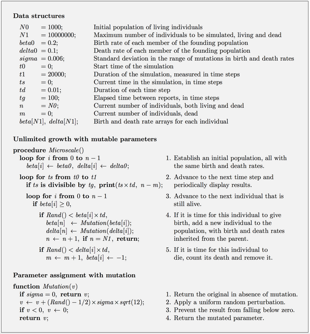
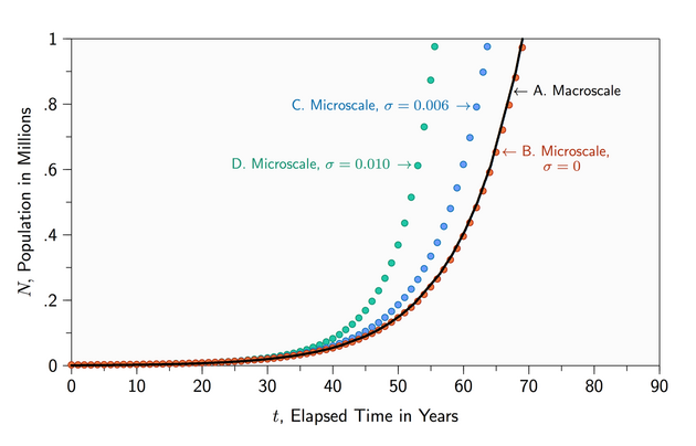
To relax other assumptions, researchers have applied computational methods. Figure 2 is a sample computational microscale algorithm that corresponds to the macroscale model of Figure 1. When all individuals are identical and mutations in birth and death rates are disabled, the microscale dynamics closely parallel the macroscale dynamics (Figures 3A and 3B). The slight differences between the two models arise from stochastic variations in the microscale version not present in the deterministic macroscale model. These variations will be different each time the algorithm is carried out, arising from intentional variations in random number sequences.
When not all individuals are identical, the microscale dynamics can differ significantly from the macroscale dynamics, simulating more realistic situations than can be modeled at the macroscale (Figures 3C and 3D). The microscale model does not explicitly incorporate the differential equation, though for large populations it simulates it closely. When individuals differ from one another, the system has a well-defined behavior but the differential equations governing that behavior are difficult to codify. The algorithm of Figure 2 is a basic example of what is called an equation-free model.[20]
When mutations are enabled in the microscale model (), the population grows more rapidly than in the macroscale model (Figures 3C and 3D). Mutations in parameters allow some individuals to have higher birth rates and others to have lower death rates, and those individuals contribute proportionally more to the population. All else being equal, the average birth rate drifts to higher values and the average death rate drifts to lower values as the simulation progresses. This drift is tracked in the data structures named beta and delta of the microscale algorithm of Figure 2.
The algorithm of Figure 2 is a simplified microscale model using the Euler method. Other algorithms such as the Gillespie method[21] and the discrete event method[17] are also used in practice. Versions of the algorithm in practical use include efficiencies such as removing individuals from consideration once they die (to reduce memory requirements and increase speed) and scheduling stochastic events into the future (to provide a continuous time scale and to further improve speed).[17] Such approaches can be orders of magnitude faster.
Complexity
The complexity of systems addressed by microscale models leads to complexity in the models themselves, and the specification of a microscale model can be tens or hundreds of times larger than its corresponding macroscale model. (The simplified example of Figure 2 has 25 times as many lines in its specification as does Figure 1.) Since bugs occur in computer software and cannot completely be removed by standard methods such as testing,[22] and since complex models often are neither published in detail nor peer-reviewed, their validity has been called into question.[23] Guidelines on best practices for microscale models exist[24] but no papers on the topic claim a full resolution of the problem of validating complex models.
Future
Computing capacity is reaching levels where populations of entire countries or even the entire world are within the reach of microscale models, and improvements in the census and travel data allow further improvements in parameterizing such models. Remote sensors from Earth-observing satellites and ground-based observatories such as the National Ecological Observatory Network (NEON) provide large amounts of data for calibration. Potential applications range from predicting and reducing the spread of disease to helping understand the dynamics of the earth.
Figures

Figure 1. One of the simplest of macroscale models: an ordinary differential equation describing continuous exponential growth. is the size of the population at the time and is the rate of change through time in a single dimension . is the initial population, is the birth rate per time unit, and is a death rate per time unit. At the left is the differential form; at the right is the explicit solution in terms of standard mathematical functions, which follows in this case from the differential form. Almost all macroscale models are more complex than this example, in that they have multiple dimensions, lack explicit solutions in terms of standard mathematical functions, and must be understood from their differential forms.

Figure 2. A basic algorithm applying the Euler method to an individual-based model. See text for discussion. The algorithm, represented in pseudocode, begins with invocation of procedure , which uses the data structures to carry out the simulation according to the numbered steps described at the right. It repeatedly invokes function , which returns its parameter perturbed by a random number drawn from a uniform distribution with standard deviation defined by the variable . (The square root of 12 appears because the standard deviation of a uniform distribution includes that factor.) Function in the algorithm is assumed to return a uniformly distributed random number . The data are assumed to be reset to their initial values on each invocation of .

Figure 3. Graphical comparison of the dynamics of macroscale and microscale simulations of Figures 1 and 2, respectively.
- (A) The black curve plots the exact solution to the macroscale model of Figure 1 with per year, per year, and individuals.
- (B) Red dots show the dynamics of the microscale model of Figure 2, shown at intervals of one year, using the same values of , , and , and with no mutations .
- (C) Blue dots show the dynamics of the microscale model with mutations having a standard deviation of .
- (D) Green dots show results with larger mutations, .
References
- ↑ Nelson, Michael France (2014). Experimental and simulation studies of the population genetics, drought tolerance, and vegetative growth of Phalaris arundinacea (Doctoral Dissertation). University of Minnesota, USA.
- ↑ Gustafsson, Leif; Sternad, Mikael (2010). "Consistent micro, macro, and state-based population modelling". Mathematical Biosciences 225 (2): 94–107. doi:10.1016/j.mbs.2010.02.003. PMID 20171974.
- ↑ Gustafsson, Leif; Sternad, Mikael (2007). "Bringing consistency to simulation of population models: Poisson Simulation as a bridge between micro and macro simulation". Mathematical Biosciences 209 (2): 361–385. doi:10.1016/j.mbs.2007.02.004. PMID 17412368. http://www.signal.uu.se/Publications/pdf/p0704.pdf.
- ↑ Dillon, Robert (1996). "Modeling biofilm processes using the immersed boundary method". Journal of Computational Physics 129 (1): 57–73. doi:10.1006/jcph.1996.0233. Bibcode: 1996JCoPh.129...57D.
- ↑ 5.0 5.1 Bandini, Stefania; Luca Federici, Mizar; Manzoni, Sara (2007). "SCA approach to microscale modelling of paradigmatic emergent crowd behaviors". SCSC: 1051–1056.
- ↑ Gartley, M. G.; Schott, J. R.; Brown, S. D. (2008). Shen, Sylvia S; Lewis, Paul E. eds. "Micro-scale modeling of contaminant effects on surface optical properties". Optical Engineering Plus Applications, International Society for Optics and Photonics. Imaging Spectrometry XIII 7086: 70860H. doi:10.1117/12.796428. Bibcode: 2008SPIE.7086E..0HG.
- ↑ 7.0 7.1 O'Sullivan, David (2002). "Toward microscale spatial modeling of gentrification". Journal of Geographical Systems 4 (3): 251–274. doi:10.1007/s101090200086. Bibcode: 2002JGS.....4..251O.
- ↑ 8.0 8.1 Less, G. B.; Seo, J. H.; Han, S.; Sastry, A. M.; Zausch, J.; Latz, A.; Schmidt, S.; Wieser, C. et al. (2012). "Microscale modeling of Li-Ion batteries: Parameterization and validation". Journal of the Electrochemical Society 159 (6): A697–A704. doi:10.1149/2.096205jes.
- ↑ 9.0 9.1 9.2 Knutz, R.; Khatib, I.; Moussiopoulos, N. (2000). "Coupling of mesoscale and microscale models—an approach to simulate scale interaction". Environmental Modelling and Software 15 (6–7): 597–602. doi:10.1016/s1364-8152(00)00055-4. Bibcode: 2000EnvMS..15..597K.
- ↑ Marchisio, Daniele L.; Fox, Rodney O. (2013). Computational models for polydisperse particulate and multiphase systems. Cambridge University Press.
- ↑ Barnes, Richard; Lehman, Clarence; Mulla, David (2014). "An efficient assignment of drainage direction over flat surfaces in raster digital elevation models". Computers and Geosciences 62: 128–135. doi:10.1016/j.cageo.2013.01.009. Bibcode: 2014CG.....62..128B.
- ↑ You, Yong; Nikolaou, Michael (1993). "Dynamic process modeling with recurrent neural networks". AIChE Journal 39 (10): 1654–1667. doi:10.1002/aic.690391009. Bibcode: 1993AIChE..39.1654Y.
- ↑ Turing, Alan M. (1952). "The chemical basis of morphogenesis". Philosophical Transactions of the Royal Society of London B: Biological Sciences 237 (641): 37–72. doi:10.1098/rstb.1952.0012. Bibcode: 1952RSPTB.237...37T.
- ↑ Burks, A. W. (1966). Theory of self-reproducing automata. University of Illinois Press. https://archive.org/details/theoryofselfrepr00vonn_0.
- ↑ Moore, Gordon E. (1965). "Cramming more components onto integrated circuits". Electronics 38 (8).
- ↑ Berezin, A. A.; Ibrahim, A. M. (2004). "Reliability of Moore's Law: A measure of maintained quality". in G. J. McNulty. Quality, Reliability and Maintenance. John Wiley and Sons.
- ↑ 17.0 17.1 17.2 Brown, Randy (1988). "Calendar Queues: A fast O(1) priority queue implementation for the simulation event set problem". Communications of the ACM 31 (10): 1220–1227. doi:10.1145/63039.63045.
- ↑ Frind, E. O.; Sudicky, E. A.; Schellenberg, S. L. (1987). "Microscale modelling in the study of plume evolution in heterogeneous media". Stochastic Hydrology and Hydraulics 1 (4): 263–279. doi:10.1007/bf01543098. Bibcode: 1987SHH.....1..263F.
- ↑ May, Robert (1974). "Stability and complexity in model ecosystems". Monographs in Population Biology (Princeton University Press) 6: 114–117. PMID 4723571.
- ↑ Kevrekidis, Ioannis G.; Samaey, Giovanni (2009). "Equation-free multiscale computation: Algorithms and applications". Annual Review of Physical Chemistry 60: 321–344. doi:10.1146/annurev.physchem.59.032607.093610. PMID 19335220. Bibcode: 2009ARPC...60..321K.
- ↑ Gillespie, Daniel T. (1977). "Exact stochastic simulation of coupled chemical reactions". Journal of Physical Chemistry 81 (25): 2340–2361. doi:10.1021/j100540a008.
- ↑ Dijkstra, Edsger (1970). Notes on structured programming. T.H. Report 70-WSK-03, EWD249. Eindhoven, The Netherlands: Technological University.
- ↑ Saltelli, Andrea; Funtowicz, Silvio (2014). "When all models are wrong". Issues in Science and Technology 30 (2): 79–85.
- ↑ Baxter, Susan M.; Day, Steven W.; Fetrow, Jacquelyn S.; Reisinger, Stephanie J. (2006). "Scientific software development is not an oxymoron". PLOS Computational Biology 2 (9): 975–978. doi:10.1371/journal.pcbi.0020087. PMID 16965174. Bibcode: 2006PLSCB...2...87B.
 |
