Multilevel Monte Carlo method

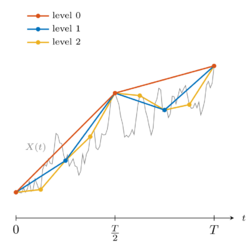
Multilevel Monte Carlo (MLMC) methods in numerical analysis are algorithms for computing expectations that arise in stochastic simulations. Just as Monte Carlo methods, they rely on repeated random sampling, but these samples are taken on different levels of accuracy. MLMC methods can greatly reduce the computational cost of standard Monte Carlo methods by taking most samples with a low accuracy and corresponding low cost, and only very few samples are taken at high accuracy and corresponding high cost.

Goal

The goal of a multilevel Monte Carlo method is to approximate the expected value [math]\displaystyle{ \operatorname{E}[G] }[/math] of the random variable [math]\displaystyle{ G }[/math] that is the output of a stochastic simulation. Suppose this random variable cannot be simulated exactly, but there is a sequence of approximations [math]\displaystyle{ G_0, G_1, \ldots, G_L }[/math] with increasing accuracy, but also increasing cost, that converges to [math]\displaystyle{ G }[/math] as [math]\displaystyle{ L\rightarrow\infty }[/math]. The basis of the multilevel method is the telescoping sum identity,

[math]\displaystyle{ \operatorname{E}[G_{L}] = \operatorname{E}[G_{0}] + \sum_{\ell=1}^L \operatorname{E}[G_\ell - G_{\ell-1}], }[/math]

that is trivially satisfied because of the linearity of the expectation operator. Each of the expectations [math]\displaystyle{ \operatorname{E}[G_\ell - G_{\ell-1}] }[/math] is then approximated by a Monte Carlo method, resulting in the multilevel Monte Carlo method. Note that taking a sample of the difference [math]\displaystyle{ G_\ell - G_{\ell-1} }[/math] at level [math]\displaystyle{ \ell }[/math] requires a simulation of both [math]\displaystyle{ G_{\ell} }[/math] and [math]\displaystyle{ G_{\ell-1} }[/math].

The MLMC method works if the variances [math]\displaystyle{ \operatorname{V}[G_\ell - G_{\ell-1}]\rightarrow0 }[/math] as [math]\displaystyle{ \ell\rightarrow\infty }[/math], which will be the case if both [math]\displaystyle{ G_{\ell} }[/math] and [math]\displaystyle{ G_{\ell-1} }[/math] approximate the same random variable [math]\displaystyle{ G }[/math]. By the Central Limit Theorem, this implies that one needs fewer and fewer samples to accurately approximate the expectation of the difference [math]\displaystyle{ G_\ell - G_{\ell-1} }[/math] as [math]\displaystyle{ \ell\rightarrow\infty }[/math]. Hence, most samples will be taken on level [math]\displaystyle{ 0 }[/math], where samples are cheap, and only very few samples will be required at the finest level [math]\displaystyle{ L }[/math]. In this sense, MLMC can be considered as a recursive control variate strategy.

Applications

Approximation of a sample path of an SDE on different levels.

The first application of MLMC is attributed to Mike Giles, in the context of stochastic differential equations (SDEs) for option pricing, however, earlier traces are found in the work of Heinrich in the context of parametric integration. Here, the random variable [math]\displaystyle{ G=f(X(T)) }[/math] is known as the payoff function, and the sequence of approximations [math]\displaystyle{ G_\ell }[/math], [math]\displaystyle{ \ell=0,\ldots,L }[/math] use an approximation to the sample path [math]\displaystyle{ X(t) }[/math] with time step [math]\displaystyle{ h_\ell=2^{-\ell}T }[/math].

The application of MLMC to problems in uncertainty quantification (UQ) is an active area of research. An important prototypical example of these problems are partial differential equations (PDEs) with random coefficients. In this context, the random variable [math]\displaystyle{ G }[/math] is known as the quantity of interest, and the sequence of approximations corresponds to a discretization of the PDE with different mesh sizes.

An algorithm for MLMC simulation

A simple level-adaptive algorithm for MLMC simulation is given below in pseudo-code.

[math]\displaystyle{ L\gets0 }[/math]
repeat
    Take warm-up samples at level [math]\displaystyle{ L }[/math]
    Compute the sample variance on all levels [math]\displaystyle{ \ell=0,\ldots,L }[/math]
    Define the optimal number of samples [math]\displaystyle{ N_\ell }[/math] on all levels [math]\displaystyle{ \ell=0,\ldots,L }[/math]
    Take additional samples on each level [math]\displaystyle{ \ell }[/math] according to [math]\displaystyle{ N_\ell }[/math]
    if [math]\displaystyle{ L\geq2 }[/math] then
        Test for convergence
    end
    if not converged then
        [math]\displaystyle{ L\gets L+1 }[/math]
    end
until converged

Extensions of MLMC

Recent extensions of the multilevel Monte Carlo method include multi-index Monte Carlo, where more than one direction of refinement is considered, and the combination of MLMC with the Quasi-Monte Carlo method.

See also

• Monte Carlo method
• Monte Carlo methods in finance
• Quasi-Monte Carlo methods in finance
• Uncertainty quantification
• Partial differential equations with random coefficients

References

- ↑ Giles, M. B. (2015). "Multilevel Monte Carlo Methods". Acta Numerica 24: 259–328. doi:10.1017/s096249291500001x.
- ↑ Giles, M. B. (2008). "Multilevel Monte Carlo Path Simulation". Operations Research 56 (3): 607–617. doi:10.1287/opre.1070.0496. https://ora.ox.ac.uk/objects/uuid:d9d28973-94aa-4179-962a-28bcfa8d8f00/datastreams/ATTACHMENT01.
- ↑ Heinrich, S. (2001). "Multilevel Monte Carlo Methods". Large-Scale Scientific Computing. Lecture Notes in Computer Science. 2179. Springer. pp. 58–67. doi:10.1007/3-540-45346-6_5. ISBN 978-3-540-43043-8.
- ↑ Cliffe, A.; Giles, M. B.; Scheichl, R.; Teckentrup, A. (2011). "Multilevel Monte Carlo Methods and Applications to Elliptic PDEs with Random Coefficients". Computing and Visualization in Science 14 (1): 3–15. doi:10.1007/s00791-011-0160-x. http://people.maths.ox.ac.uk/~gilesm/files/cgst.pdf.
- ↑ Pisaroni, M.; Nobile, F. B.; Leyland, P. (2017). "A Continuation Multi Level Monte Carlo Method for Uncertainty Quantification in Compressible Inviscid Aerodynamics". Computer Methods in Applied Mechanics and Engineering 326 (C): 20–50. doi:10.1016/j.cma.2017.07.030. https://pdfs.semanticscholar.org/6dbc/8dde601b1757c42a4c54fa9cfd69317c82c8.pdf.
- ↑ Haji-Ali, A. L.; Nobile, F.; Tempone, R. (2016). "Multi-Index Monte Carlo: When Sparsity Meets Sampling". Numerische Mathematik 132 (4): 767–806. doi:10.1007/s00211-015-0734-5.
- ↑ Giles, M. B.; Waterhouse, B. (2009). "Multilevel Quasi-Monte Carlo Path Simulation". Advanced Financial Modelling, Radon Series on Computational and Applied Mathematics (De Gruyter): 165–181. http://people.maths.ox.ac.uk/gilesm/files/jcf07.pdf.
- ↑ Robbe, P.; Nuyens, D.; Vandewalle, S. (2017). "A Multi-Index Quasi-Monte Carlo Algorithm for Lognormal Diffusion Problems". SIAM Journal on Scientific Computing 39 (5): A1811–C392. doi:10.1137/16M1082561. Bibcode: 2017SJSC...39S.851R.