Pruning (morphology)
The pruning algorithm is a technique used in digital image processing based on mathematical morphology.[1] It is used as a complement to the skeleton and thinning algorithms to remove unwanted parasitic components (spurs). In this case 'parasitic' components refer to branches of a line which are not key to the overall shape of the line and should be removed. These components can often be created by edge detection algorithms or digitization. Common uses for pruning include automatic recognition of hand-printed characters. Often inconsistency in letter writing creates unwanted spurs that need to be eliminated for better characterization.[2]
Mathematical Definition
The standard pruning algorithm will remove all branches shorter than a given number of points. If a parasitic branch is shorter than four points and we run the algorithm with n = 4 the branch will be removed. The second step ensures that the main trunks of each line are not shortened by the procedure.
Structuring Elements
The x in the arrays indicates a “don’t care” condition i.e. the image could have either a 1 or a 0 in the spot.
Step 1: Thinning
Apply this step a given (n) times to eliminate any branch with (n) or less pixels.
Step 2: Find End Points
Wherever the structuring elements are satisfied, the center of the 3x3 matrix is considered an endpoint.
Step 3: Dilate End Points
Perform dilation using a 3x3 matrix (H) consisting of all 1's and only insert 1's where the original image (A) also had a 1. Perform this for each endpoint in all direction (n) times.
Step 4: Union of X1 & X3
Take the result from step 1 and union it with step 3 to achieve the final results.
MATLAB Code
%% ---------------
% Pruning
% ---------------
clear; clc;

% Image read in
img = imread('Pruning.tif');

b_img_skel = bwmorph (img, 'skel', 40);
b_img_spur = bwmorph(b_img_skel, 'spur', Inf);

figure('Name', 'Pruning');
subplot(1,2,1);
imshow(b_img_skel);
title(sprintf('Image Skeleton'));
subplot(1,2,2);
imshow(b_img_spur);
title(sprintf('Skeleton Image Pruned'));
MATLAB Example
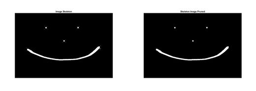
In the MATLAB example below, it takes the original image (below left) and skeletonize it 40 times then prunes the image to remove the spurs as per the MATLAB code above. As shown (below right) this removed the majority of all spurs resulting in a cleaner image.
| Original Image | Image Skeleton | Skeleton Image Pruned |
|---|---|---|
| File:Pruning.tif | 
| |
See also
- Morphological image processing
External links
References
- ↑ Russ, John C. (2011). The image processing handbook (6th ed.). Boca Raton: CRC Press. ISBN 978-1-4398-4045-0.
- ↑ Gonzalez, Rafael C.; Woods, Richard E. (2008). Digital image processing (3rd ed.). Upper Saddle River, N.J.: Prentice Hall. ISBN 978-0131687288.
 |
