Shifted log-logistic distribution

Shifted log-logistic

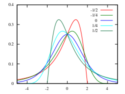
Probability density function [math]\displaystyle{ \mu=0, \sigma=1, }[/math] values of [math]\displaystyle{ \xi }[/math] as shown in legend
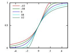
Cumulative distribution function [math]\displaystyle{ \mu=0, \sigma=1, }[/math] values of [math]\displaystyle{ \xi }[/math] as shown in legend
Parameters	[math]\displaystyle{ \mu \in (-\infty,+\infty) \, }[/math] location (real) [math]\displaystyle{ \sigma \in (0,+\infty) \, }[/math] scale (real) [math]\displaystyle{ \xi\in (-\infty,+\infty) \, }[/math] shape (real)
Support	[math]\displaystyle{ x \geqslant \mu -\sigma/\xi\,\;(\xi \gt 0) }[/math] [math]\displaystyle{ x \leqslant \mu -\sigma/\xi\,\;(\xi \lt 0) }[/math] [math]\displaystyle{ x \in (-\infty, +\infty) \,\;(\xi = 0) }[/math]
PDF	[math]\displaystyle{ \frac{(1+\xi z)^{-(1/\xi +1)}}{\sigma\left(1 + (1+\xi z)^{-1/\xi}\right)^2} }[/math] where [math]\displaystyle{ z=(x-\mu)/\sigma\, }[/math]
CDF	[math]\displaystyle{ \left(1+(1 + \xi z)^{-1/\xi}\right)^{-1} \, }[/math] where [math]\displaystyle{ z=(x-\mu)/\sigma\, }[/math]
Mean	[math]\displaystyle{ \mu + \frac{\sigma}{\xi}(\alpha \csc(\alpha)-1) }[/math] where [math]\displaystyle{ \alpha= \pi \xi\, }[/math]
Median	[math]\displaystyle{ \mu \, }[/math]
Mode	[math]\displaystyle{ \mu + \frac{\sigma}{\xi}\left[\left(\frac{1-\xi}{1+\xi}\right)^\xi - 1 \right] }[/math]
Variance	[math]\displaystyle{ \frac{\sigma^2}{\xi^2}[2\alpha \csc(2 \alpha) - (\alpha \csc(\alpha))^2] }[/math] where [math]\displaystyle{ \alpha= \pi \xi\, }[/math]

The shifted log-logistic distribution is a probability distribution also known as the generalized log-logistic or the three-parameter log-logistic distribution. It has also been called the generalized logistic distribution, but this conflicts with other uses of the term: see generalized logistic distribution.

Definition

The shifted log-logistic distribution can be obtained from the log-logistic distribution by addition of a shift parameter [math]\displaystyle{ \delta }[/math]. Thus if [math]\displaystyle{ X }[/math] has a log-logistic distribution then [math]\displaystyle{ X+\delta }[/math] has a shifted log-logistic distribution. So [math]\displaystyle{ Y }[/math] has a shifted log-logistic distribution if [math]\displaystyle{ \log(Y-\delta) }[/math] has a logistic distribution. The shift parameter adds a location parameter to the scale and shape parameters of the (unshifted) log-logistic.

The properties of this distribution are straightforward to derive from those of the log-logistic distribution. However, an alternative parameterisation, similar to that used for the generalized Pareto distribution and the generalized extreme value distribution, gives more interpretable parameters and also aids their estimation.

In this parameterisation, the cumulative distribution function (CDF) of the shifted log-logistic distribution is

[math]\displaystyle{ F(x; \mu,\sigma,\xi) = \frac{1}{ 1 + \left(1+ \frac{\xi(x-\mu)}{\sigma}\right)^{-1/\xi}} }[/math]

for [math]\displaystyle{ 1 + \xi(x-\mu)/\sigma \geqslant 0 }[/math], where [math]\displaystyle{ \mu\in\mathbb R }[/math] is the location parameter, [math]\displaystyle{ \sigma\gt 0\, }[/math] the scale parameter and [math]\displaystyle{ \xi\in\mathbb R }[/math] the shape parameter. Note that some references use [math]\displaystyle{ \kappa = - \xi\,\! }[/math] to parameterise the shape.

The probability density function (PDF) is

[math]\displaystyle{ f(x; \mu,\sigma,\xi) = \frac{\left(1+\frac{\xi(x-\mu)}{\sigma}\right)^{-(1/\xi +1)}} {\sigma\left[1 + \left(1+\frac{\xi(x-\mu)}{\sigma}\right)^{-1/\xi}\right]^2}, }[/math]

again, for [math]\displaystyle{ 1 + \xi(x-\mu)/\sigma \geqslant 0. }[/math]

The shape parameter [math]\displaystyle{ \xi }[/math] is often restricted to lie in [-1,1], when the probability density function is bounded. When [math]\displaystyle{ |\xi|\gt 1 }[/math], it has an asymptote at [math]\displaystyle{ x = \mu - \sigma/\xi }[/math]. Reversing the sign of [math]\displaystyle{ \xi }[/math] reflects the pdf and the cdf about [math]\displaystyle{ x=\mu. }[/math].

Related distributions

• When [math]\displaystyle{ \mu = \sigma/\xi, }[/math] the shifted log-logistic reduces to the log-logistic distribution.
• When [math]\displaystyle{ \xi }[/math] → 0, the shifted log-logistic reduces to the logistic distribution.
• The shifted log-logistic with shape parameter [math]\displaystyle{ \xi=1 }[/math] is the same as the generalized Pareto distribution with shape parameter [math]\displaystyle{ \xi=1. }[/math]

Applications

The three-parameter log-logistic distribution is used in hydrology for modelling flood frequency.

Alternate parameterization

An alternate parameterization with simpler expressions for the PDF and CDF is as follows. For the shape parameter [math]\displaystyle{ \alpha }[/math], scale parameter [math]\displaystyle{ \beta }[/math] and location parameter [math]\displaystyle{ \gamma }[/math], the PDF is given by

[math]\displaystyle{ f(x) = \frac{\alpha}{\beta} \bigg(\frac{x-\gamma}{\beta} \bigg) ^{\alpha -1}\bigg(1+\bigg(\frac{x-\gamma}{\beta}\bigg)^\alpha\bigg)^{-2} }[/math]

The CDF is given by

[math]\displaystyle{ F(x) = \bigg(1+\bigg(\frac{\beta}{x-\gamma}\bigg)^\alpha\bigg)^{-1} }[/math]

The mean is [math]\displaystyle{ \beta \theta \csc(\theta) + \gamma }[/math] and the variance is [math]\displaystyle{ \beta^2\theta[2\csc(2\theta)-\theta \csc^2(\theta)] }[/math], where [math]\displaystyle{ \theta = \frac{\pi}{\alpha} }[/math].

References

- ↑ Venter, Gary G. (Spring 1994), "Introduction to selected papers from the variability in reserves prize program", Casualty Actuarial Society Forum 1: 91–101, http://www.casact.org/pubs/forum/94spforum/94spf091.pdf
- ↑ Geskus, Ronald B. (2001), "Methods for estimating the AIDS incubation time distribution when date of seroconversion is censored", Statistics in Medicine 20 (5): 795–812, doi:10.1002/sim.700, PMID 11241577
- ↑ 3.0 3.1 3.2 Hosking, Jonathan R. M.; Wallis, James R (1997), Regional Frequency Analysis: An Approach Based on L-Moments, Cambridge University Press, ISBN 0-521-43045-3
- ↑ 4.0 4.1 Robson, A.; Reed, D. (1999), Flood Estimation Handbook, 3: "Statistical Procedures for Flood Frequency Estimation", Wallingford, UK: Institute of Hydrology, ISBN 0-948540-89-3
- ↑ Ahmad, M. I.; Sinclair, C. D.; Werritty, A. (1988), "Log-logistic flood frequency analysis", Journal of Hydrology 98 (3–4): 205–224, doi:10.1016/0022-1694(88)90015-7, Bibcode: 1988JHyd...98..205A
- ↑ "EasyFit - Log-Logistic Distribution". http://www.mathwave.com/help/easyfit/html/analyses/distributions/log-logistic.html.
- ↑ 7.0 7.1 "Guide to Using - RISK7_EN.pdf". http://www.palisade.com/downloads/documentation/75/EN/RISK7_EN.pdf.