Generalized logistic distribution

Short description: Name for several different families of probability distributions

The term generalized logistic distribution is used as the name for several different families of probability distributions. For example, Johnson et al. list four forms, which are listed below.

Type I has also been called the skew-logistic distribution. Type IV subsumes the other types and is obtained when applying the logit transform to beta random variates. Following the same convention as for the log-normal distribution, type IV may be referred to as the logistic-beta distribution, with reference to the standard logistic function, which is the inverse of the logit transform.

For other families of distributions that have also been called generalized logistic distributions, see the shifted log-logistic distribution, which is a generalization of the log-logistic distribution; and the metalog ("meta-logistic") distribution, which is highly shape-and-bounds flexible and can be fit to data with linear least squares.

Definitions

The following definitions are for standardized versions of the families, which can be expanded to the full form as a location-scale family. Each is defined using either the cumulative distribution function (F) or the probability density function (ƒ), and is defined on (-∞,∞).

Type I

[math]\displaystyle{ F(x;\alpha)=\frac{1}{(1+e^{-x})^\alpha} \equiv (1+e^{-x})^{-\alpha}, \quad \alpha \gt 0 . }[/math]

The corresponding probability density function is:

[math]\displaystyle{ f(x;\alpha)=\frac{\alpha e^{-x}}{\left(1+e^{-x}\right)^{\alpha+1}}, \quad \alpha \gt 0 . }[/math]

This type has also been called the "skew-logistic" distribution.

Type II

[math]\displaystyle{ F(x;\alpha)=1-\frac{e^{-\alpha x}}{(1+e^{-x})^\alpha}, \quad \alpha \gt 0 . }[/math]

The corresponding probability density function is:

[math]\displaystyle{ f(x;\alpha)=\frac{\alpha e^{-\alpha x}}{(1+e^{-x})^{\alpha+1}}, \quad \alpha \gt 0 . }[/math]

Type III

[math]\displaystyle{ f(x;\alpha)=\frac{1}{B(\alpha,\alpha)}\frac{e^{-\alpha x}}{(1+e^{-x})^{2\alpha}}, \quad \alpha \gt 0 . }[/math]

Here B is the beta function. The moment generating function for this type is

[math]\displaystyle{ M(t)=\frac{\Gamma(\alpha-t) \Gamma(\alpha+t) }{ (\Gamma(\alpha))^2 }, \quad -\alpha\lt t\lt \alpha. }[/math]

The corresponding cumulative distribution function is:

[math]\displaystyle{ F(x;\alpha)= \frac{\left(e^x+1\right) \Gamma (\alpha ) e^{\alpha (-x)} \left(e^{-x}+1\right)^{-2 \alpha } \, _2\tilde{F}_1\left(1,1-\alpha ;\alpha +1;-e^x\right)}{B(\alpha ,\alpha )}, \quad \alpha \gt 0 . }[/math]

Type IV

[math]\displaystyle{ \begin{align} f(x;\alpha,\beta)&=\frac{1}{B(\alpha,\beta)}\frac{e^{-\beta x}}{(1+e^{-x})^{\alpha+\beta}}, \quad \alpha,\beta \gt 0 \\[4pt] &= \frac{\sigma(x)^\alpha\sigma(-x)^\beta}{B(\alpha,\beta)} . \end{align} }[/math]

Where, B is the beta function and [math]\displaystyle{ \sigma(x)=1/(1+e^{-x}) }[/math] is the standard logistic function. The moment generating function for this type is

[math]\displaystyle{ M(t)=\frac{\Gamma(\beta-t) \Gamma(\alpha+t) }{ \Gamma(\alpha) \Gamma(\beta) }, \quad -\alpha\lt t\lt \beta. }[/math]

This type is also called the "exponential generalized beta of the second type".

The corresponding cumulative distribution function is:

[math]\displaystyle{ F(x;\alpha,\beta)= \frac{\left(e^x+1\right) \Gamma (\alpha ) e^{\beta (-x)} \left(e^{-x}+1\right)^{-\alpha -\beta } \, _2\tilde{F}_1\left(1,1-\beta ;\alpha +1;-e^x\right)}{B(\alpha ,\beta )} , \quad \alpha,\beta \gt 0 . }[/math]

Relationship between types

Type IV is the most general form of the distribution. The Type III distribution can be obtained from Type IV by fixing [math]\displaystyle{ \beta = \alpha }[/math]. The Type II distribution can be obtained from Type IV by fixing [math]\displaystyle{ \alpha = 1 }[/math] (and renaming [math]\displaystyle{ \beta }[/math] to [math]\displaystyle{ \alpha }[/math]). The Type I distribution can be obtained from Type IV by fixing [math]\displaystyle{ \beta = 1 }[/math]. Fixing [math]\displaystyle{ \alpha=\beta=1 }[/math] gives the standard logistic distribution.

Type IV (logistic-beta) properties

Type IV probability density functions (means=0, variances=1)

The Type IV generalized logistic, or logistic-beta distribution, with support [math]\displaystyle{ x\in\mathbb{R} }[/math] and shape parameters [math]\displaystyle{ \alpha,\beta\gt 0 }[/math], has (as shown above) the probability density function (pdf):

[math]\displaystyle{ f(x;\alpha,\beta)= \frac{1}{B(\alpha,\beta)}\frac{e^{-\beta x}}{(1+e^{-x})^{\alpha+\beta}} = \frac{\sigma(x)^\alpha\sigma(-x)^\beta}{B(\alpha,\beta)}, }[/math]

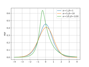
where [math]\displaystyle{ \sigma(x)=1/(1+e^{-x}) }[/math] is the standard logistic function. The probability density functions for three different sets of shape parameters are shown in the plot, where the distributions have been scaled and shifted to give zero means and unity variances, in order to facilitate comparison of the shapes.

In what follows, the notation [math]\displaystyle{ B_\sigma(\alpha,\beta) }[/math] is used to denote the Type IV distribution.

Relationship with Gamma Distribution

This distribution can be obtained in terms of the gamma distribution as follows. Let [math]\displaystyle{ y\sim\text{Gamma}(\alpha,\gamma) }[/math] and independently, [math]\displaystyle{ z\sim\text{Gamma}(\beta,\gamma) }[/math] and let [math]\displaystyle{ x=\ln y - \ln z }[/math]. Then [math]\displaystyle{ x\sim B_\sigma(\alpha,\beta) }[/math].

Symmetry

If [math]\displaystyle{ x\sim B_\sigma(\alpha,\beta) }[/math], then [math]\displaystyle{ -x\sim B_\sigma(\beta,\alpha) }[/math].

Mean and variance

By using the logarithmic expectations of the gamma distribution, the mean and variance can be derived as:

[math]\displaystyle{ \begin{align} \text{E}[x] &= \psi(\alpha) - \psi(\beta) \\ \text{var}[x] &= \psi'(\alpha) + \psi'(\beta) \\ \end{align} }[/math]

where [math]\displaystyle{ \psi }[/math] is the digamma function, while [math]\displaystyle{ \psi'=\psi^{(1)} }[/math] is its first derivative, also known as the trigamma function, or the first polygamma function. Since [math]\displaystyle{ \psi }[/math] is strictly increasing, the sign of the mean is the same as the sign of [math]\displaystyle{ \alpha-\beta }[/math]. Since [math]\displaystyle{ \psi' }[/math] is strictly decreasing, the shape parameters can also be interpreted as concentration parameters. Indeed, as shown below, the left and right tails respectively become thinner as [math]\displaystyle{ \alpha }[/math] or [math]\displaystyle{ \beta }[/math] are increased. The two terms of the variance represent the contributions to the variance of the left and right parts of the distribution.

Cumulants and skewness

The cumulant generating function is [math]\displaystyle{ K(t)=\ln M(t) }[/math], where the moment generating function [math]\displaystyle{ M(t) }[/math] is given above. The cumulants, [math]\displaystyle{ \kappa_n }[/math], are the [math]\displaystyle{ n }[/math]-th derivatives of [math]\displaystyle{ K(t) }[/math], evaluated at [math]\displaystyle{ t=0 }[/math]:

[math]\displaystyle{ \kappa_n = K^{(n)}(0) = \psi^{(n-1)}(\alpha) + (-1)^{n} \psi^{(n-1)}(\beta) }[/math]

where [math]\displaystyle{ \psi^{(0)}=\psi }[/math] and [math]\displaystyle{ \psi^{(n-1)} }[/math] are the digamma and polygamma functions. In agreement with the derivation above, the first cumulant, [math]\displaystyle{ \kappa_1 }[/math], is the mean and the second, [math]\displaystyle{ \kappa_2 }[/math], is the variance.

The third cumulant, [math]\displaystyle{ \kappa_3 }[/math], is the third central moment [math]\displaystyle{ E[(x-E[x])^3] }[/math], which when scaled by the third power of the standard deviation gives the skewness:

[math]\displaystyle{ \text{skew}[x] = \frac{\psi^{(2)}(\alpha) - \psi^{(2)}(\beta)}{\sqrt{\text{var}[x]}^3} }[/math]

The sign (and therefore the handedness) of the skewness is the same as the sign of [math]\displaystyle{ \alpha-\beta }[/math].

Mode

The mode (pdf maximum) can be derived by finding [math]\displaystyle{ x }[/math] where the log pdf derivative is zero:

[math]\displaystyle{ \frac{d}{dx}\ln f(x;\alpha,\beta) = \alpha\sigma(-x) -\beta\sigma(x) = 0 }[/math]

This simplifies to [math]\displaystyle{ \alpha/\beta=e^x }[/math], so that:

[math]\displaystyle{ \text{mode}[x] = \ln\frac{\alpha}{\beta} }[/math]

Tail behaviour

Tail comparison: Type IV (means=0, variances=1) vs standard normal, vs standard Cauchy

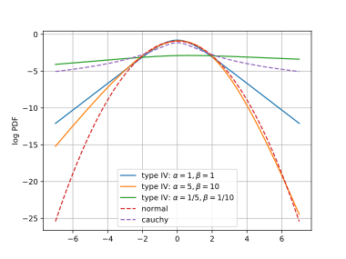
In each of the left and right tails, one of the sigmoids in the pdf saturates to one, so that the tail is formed by the other sigmoid. For large negative [math]\displaystyle{ x }[/math], the left tail of the pdf is proportional to [math]\displaystyle{ \sigma(x)^\alpha\approx e^{\alpha x} }[/math], while the right tail (large positive [math]\displaystyle{ x }[/math]) is proportional to [math]\displaystyle{ \sigma(-x)^\beta\approx e^{-\beta x} }[/math]. This means the tails are independently controlled by [math]\displaystyle{ \alpha }[/math] and [math]\displaystyle{ \beta }[/math]. Although type IV tails are heavier than those of the normal distribution ([math]\displaystyle{ e^{-\frac{x^2}{2v}} }[/math], for variance [math]\displaystyle{ v }[/math]), the type IV means and variances remain finite for all [math]\displaystyle{ \alpha,\beta\gt 0 }[/math]. This is in contrast with the Cauchy distribution for which the mean and variance do not exist. In the log pdf plots shown here, the type IV tails are linear, the normal distribution tails are quadratic and the Cauchy tails are logarithmic.

Exponential family properties

[math]\displaystyle{ B_\sigma(\alpha,\beta) }[/math] forms an exponential family with natural parameters [math]\displaystyle{ \alpha }[/math] and [math]\displaystyle{ \beta }[/math] and sufficient statistics [math]\displaystyle{ \log\sigma(x) }[/math] and [math]\displaystyle{ \log\sigma(-x) }[/math]. The expected values of the sufficient statistics can be found by differentiation of the log-normalizer:

[math]\displaystyle{ \begin{align} E[\log\sigma(x)] &= \frac{\partial\log B(\alpha,\beta)}{\partial\alpha} = \psi(\alpha) - \psi(\alpha+\beta) \\ E[\log\sigma(-x)] &= \frac{\partial\log B(\alpha,\beta)}{\partial\beta} = \psi(\beta) - \psi(\alpha+\beta) \\ \end{align} }[/math]

Given a data set [math]\displaystyle{ x_1,\ldots,x_n }[/math] assumed to have been generated IID from [math]\displaystyle{ B_\sigma(\alpha,\beta) }[/math], the maximum-likelihood parameter estimate is:

[math]\displaystyle{ \begin{align} \hat\alpha,\hat\beta = \arg\max_{\alpha,\beta} &\;\frac1n\sum_{i=1}^n \log f(x_i;\alpha,\beta) \\ =\arg\max_{\alpha,\beta} &\;\alpha\Bigl(\frac1n\sum_i\log\sigma(x_i)\Bigr) + \beta\Bigl(\frac1n\sum_i\log\sigma(-x_i)\Bigr) -\log B(\alpha,\beta)\\ =\arg\max_{\alpha,\beta}&\;\alpha\,\overline{\log\sigma(x)} + \beta\,\overline{\log\sigma(-x)} -\log B(\alpha,\beta) \end{align} }[/math]

where the overlines denote the averages of the sufficient statistics. The maximum-likelihood estimate depends on the data only via these average statistics. Indeed, at the maximum-likelihood estimate the expected values and averages agree:

[math]\displaystyle{ \begin{align} \psi(\hat\alpha) - \psi(\hat\alpha+\hat\beta) &= \overline{\log\sigma(x)} \\ \psi(\hat\beta) - \psi(\hat\alpha+\hat\beta) &= \overline{\log\sigma(-x)} \\ \end{align} }[/math]

which is also where the partial derivatives of the above maximand vanish.

Relationships with other distributions

Relationships with other distributions include:

• The log-ratio of gamma variates is of type IV as detailed above.
• If [math]\displaystyle{ y\sim\text{BetaPrime}(\alpha,\beta) }[/math], then [math]\displaystyle{ x=\ln y }[/math] has a type IV distribution, with parameters [math]\displaystyle{ \alpha }[/math] and [math]\displaystyle{ \beta }[/math]. See beta prime distribution.
• If [math]\displaystyle{ z\sim\text{Gamma}(\beta,1) }[/math] and [math]\displaystyle{ y\mid z\sim\text{Gamma}(\alpha,z) }[/math], where [math]\displaystyle{ z }[/math] is used as the rate parameter of the second gamma distribution, then [math]\displaystyle{ y }[/math] has a compound gamma distribution, which is the same as [math]\displaystyle{ \text{BetaPrime}(\alpha,\beta) }[/math], so that [math]\displaystyle{ x=\ln y }[/math] has a type IV distribution.
• If [math]\displaystyle{ p\sim\text{Beta}(\alpha,\beta) }[/math], then [math]\displaystyle{ x=\text{logit}\, p }[/math] has a type IV distribution, with parameters [math]\displaystyle{ \alpha }[/math] and [math]\displaystyle{ \beta }[/math]. See beta distribution. The logit function, [math]\displaystyle{ \mathrm{logit}(p) = \log\frac{p}{1-p} }[/math] is the inverse of the logistic function. This relationship explains the name logistic-beta for this distribution: if the logistic function is applied to logistic-beta variates, the transformed distribution is beta.

Large shape parameters

Type IV vs normal distribution with matched mean and variance. For large values of [math]\displaystyle{ \alpha,\beta }[/math], the pdf's are very similar, except for very rare values of [math]\displaystyle{ x }[/math].

For large values of the shape parameters, [math]\displaystyle{ \alpha,\beta\gg1 }[/math], the distribution becomes more Gaussian, with:

[math]\displaystyle{ \begin{align} E[x]&\approx\ln\frac{\alpha}{\beta} \\ \text{var}[x] &\approx\frac{\alpha+\beta}{\alpha\beta} \end{align} }[/math]

This is demonstrated in the pdf and log pdf plots here.

Random variate generation

Since random sampling from the gamma and beta distributions are readily available on many software platforms, the above relationships with those distributions can be used to generate variates from the type IV distribution.

Generalization with location and scale parameters

A flexible, four-parameter family can be obtained by adding location and scale parameters. One way to do this is if [math]\displaystyle{ x\sim B_\sigma(\alpha,\beta) }[/math], then let [math]\displaystyle{ y=kx+\delta }[/math], where [math]\displaystyle{ k\gt 0 }[/math] is the scale parameter and [math]\displaystyle{ \delta\in\mathbb{R} }[/math] is the location parameter. The four-parameter family obtained thus has the desired additional flexibility, but the new parameters may be hard to interpret because [math]\displaystyle{ \delta\ne E[y] }[/math] and [math]\displaystyle{ k^2\ne \text{var}[y] }[/math]. Moreover maximum-likelihood estimation with this parametrization is hard. These problems can be addressed as follows.

Recall that the mean and variance of [math]\displaystyle{ x }[/math] are:

[math]\displaystyle{ \begin{align} \tilde\mu&=\psi(\alpha)-\psi(\beta), &\tilde s^2&=\psi'(\alpha)+\psi'(\beta) \end{align} }[/math]

Now expand the family with location parameter [math]\displaystyle{ \mu\in\mathbb{R} }[/math] and scale parameter [math]\displaystyle{ s\gt 0 }[/math], via the transformation:

[math]\displaystyle{ \begin{align} y&=\mu + \frac{s}{\tilde s}(x-\tilde\mu) \iff x=\tilde\mu + \frac{\tilde s}{s}(y-\mu) \end{align} }[/math]

so that [math]\displaystyle{ \mu=E[y] }[/math] and [math]\displaystyle{ s^2=\text{var}[y] }[/math] are now interpretable. It may be noted that allowing [math]\displaystyle{ s }[/math] to be either positive or negative does not generalize this family, because of the above-noted symmetry property. We adopt the notation [math]\displaystyle{ y\sim\bar B_\sigma(\alpha,\beta,\mu,s^2) }[/math] for this family.

If the pdf for [math]\displaystyle{ x\sim B_\sigma(\alpha,\beta) }[/math] is [math]\displaystyle{ f(x;\alpha,\beta) }[/math], then the pdf for [math]\displaystyle{ y\sim \bar B_\sigma(\alpha,\beta,\mu,s^2) }[/math] is:

[math]\displaystyle{ \bar f(y;\alpha,\beta,\mu,s^2) = \frac{\tilde s}{s}\, f(x;\alpha,\beta) }[/math]

where it is understood that [math]\displaystyle{ x }[/math] is computed as detailed above, as a function of [math]\displaystyle{ y,\alpha,\beta,\mu,s }[/math]. The pdf and log-pdf plots above, where the captions contain (means=0, variances=1), are for [math]\displaystyle{ \bar B_\sigma(\alpha,\beta,0,1) }[/math].

Maximum likelihood parameter estimation

In this section, maximum-likelihood estimation of the distribution parameters, given a dataset [math]\displaystyle{ x_1,\ldots,x_n }[/math] is discussed in turn for the families [math]\displaystyle{ B_\sigma(\alpha,\beta) }[/math] and [math]\displaystyle{ \bar B_\sigma(\alpha,\beta,\mu,s^2) }[/math].

Maximum likelihood for standard Type IV

As noted above, [math]\displaystyle{ B_\sigma(\alpha,\beta) }[/math] is an exponential family with natural parameters [math]\displaystyle{ \alpha,\beta }[/math], the maximum-likelihood estimates of which depend only on averaged sufficient statistics:

[math]\displaystyle{ \begin{align} \overline{\log\sigma(x)}&=\frac1n\sum_i\log\sigma(x_i) &&\text{and} & \overline{\log\sigma(-x)}&=\frac1n\sum_i\log\sigma(-x_i) \end{align} }[/math]

Once these statistics have been accumulated, the maximum-likelihood estimate is given by:

[math]\displaystyle{ \begin{align} \hat\alpha,\hat\beta =\arg\max_{\alpha,\beta\gt 0}&\;\alpha\,\overline{\log\sigma(x)} + \beta\,\overline{\log\sigma(-x)} -\log B(\alpha,\beta) \end{align} }[/math]

By using the parametrization [math]\displaystyle{ \theta_1=\log\alpha }[/math] and [math]\displaystyle{ \theta_2=\log\beta }[/math] an unconstrained numerical optimization algorithm like BFGS can be used. Optimization iterations are fast, because they are independent of the size of the data-set.

An alternative is to use an EM-algorithm based on the composition: [math]\displaystyle{ x-\log(\gamma\delta)\sim B_\sigma(\alpha,\beta) }[/math] if [math]\displaystyle{ z\sim\text{Gamma}(\beta,\gamma) }[/math] and [math]\displaystyle{ e^x\mid z\sim\text{Gamma}(\alpha,z/\delta) }[/math]. Because of the self-conjugacy of the gamma distribution, the posterior expectations, [math]\displaystyle{ \left\langle z\right\rangle_{P(z\mid x)} }[/math] and [math]\displaystyle{ \left\langle\log z\right\rangle_{P(z\mid x)} }[/math] that are required for the E-step can be computed in closed form. The M-step parameter update can be solved analogously to maximum-likelihood for the gamma distribution.

Maximum likelihood for the four-parameter family

The maximum-likelihood problem for [math]\displaystyle{ \bar B_\sigma(\alpha,\beta,\mu,s^2) }[/math], having pdf [math]\displaystyle{ \bar f }[/math] is:

[math]\displaystyle{ \hat\alpha,\hat\beta,\hat\mu,\hat s = \arg\max_{\alpha,\beta,\mu,s} \log\frac1n\sum_i \bar f(x_i;\alpha,\beta,\mu,s^2) }[/math]

This is no longer an exponential family, so that each optimization iteration has to traverse the whole data-set. Moreover the computation of the partial derivatives (as required for example by BFGS) is considerably more complex than for the above two-parameter case. However, all the component functions are readily available in software packages with automatic differentiation. Again, the positive parameters can be parametrized in terms of their logarithms to obtain an unconstrained numerical optimization problem.

For this problem, numerical optimization may fail unless the initial location and scale parameters are chosen appropriately. However the above-mentioned interpretability of these parameters in the parametrization of [math]\displaystyle{ \bar B_\sigma }[/math] can be used to do this. Specifically, the initial values for [math]\displaystyle{ \mu }[/math] and [math]\displaystyle{ s^2 }[/math] can be set to the empirical mean and variance of the data.

See also

• Champernowne distribution, another generalization of the logistic distribution.

References

- ↑ 1.0 1.1 Johnson, N.L., Kotz, S., Balakrishnan, N. (1995) Continuous Univariate Distributions, Volume 2, Wiley. ISBN 0-471-58494-0 (pages 140–142)
- ↑ 2.0 2.1 Lee, C. J., Zito, A., Sang, H., & Dunson, D. B. (2025). Logistic-Beta Processes for Dependent Random Probabilities with Beta Marginals. Bayesian Analysis, 1(1), 1-25. https://doi.org/10.1214/25-BA1541
- ↑ 3.0 3.1 Halliwell, L. J. (2021). The log-gamma distribution and non-normal error. Variance 2(13). https://www.casact.org/abstract/log-gamma-distribution-and-non-normal-error
- ↑ Barndorff-Nielsen, O., Kent, J., & Sørensen, M. (1982). Normal variance-mean mixtures and z distributions. International Statistical Review, 145-159. https://doi.org/10.2307/1402598
- ↑ C.M.Bishop, Pattern Recognition and Machine Learning, Springer 2006.