Generalized Pareto distribution

Short description: Family of probability distributions often used to model tails or extreme values

Generalized Pareto distribution

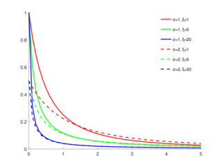
Probability density function GPD distribution functions for [math]\displaystyle{ \mu=0 }[/math] and different values of [math]\displaystyle{ \sigma }[/math] and [math]\displaystyle{ \xi }[/math]
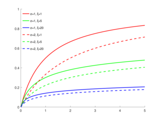
Cumulative distribution function
Parameters	[math]\displaystyle{ \mu \in (-\infty,\infty) \, }[/math] location (real) [math]\displaystyle{ \sigma \in (0,\infty) \, }[/math] scale (real) [math]\displaystyle{ \xi\in (-\infty,\infty) \, }[/math] shape (real)
Support	[math]\displaystyle{ x \geqslant \mu\,\;(\xi \geqslant 0) }[/math] [math]\displaystyle{ \mu \leqslant x \leqslant \mu-\sigma/\xi\,\;(\xi \lt 0) }[/math]
PDF	[math]\displaystyle{ \frac{1}{\sigma}(1 + \xi z )^{-(1/\xi +1)} }[/math] where [math]\displaystyle{ z=\frac{x-\mu}{\sigma} }[/math]
CDF	[math]\displaystyle{ 1-(1+\xi z)^{-1/\xi} \, }[/math]
Mean	[math]\displaystyle{ \mu + \frac{\sigma}{1-\xi}\, \; (\xi \lt 1) }[/math]
Median	[math]\displaystyle{ \mu + \frac{\sigma( 2^{\xi} -1)}{\xi} }[/math]
Mode	[math]\displaystyle{ \mu }[/math]
Variance	[math]\displaystyle{ \frac{\sigma^2}{(1-\xi)^2(1-2\xi)}\, \; (\xi \lt 1/2) }[/math]
Skewness	[math]\displaystyle{ \frac{2(1+\xi)\sqrt{1-2\xi}}{(1-3\xi)}\,\;(\xi\lt 1/3) }[/math]
Kurtosis	[math]\displaystyle{ \frac{3(1-2\xi)(2\xi^2+\xi+3)}{(1-3\xi)(1-4\xi)}-3\,\;(\xi\lt 1/4) }[/math]
Entropy	[math]\displaystyle{ \log(\sigma) + \xi + 1 }[/math]
MGF	[math]\displaystyle{ e^{\theta\mu}\,\sum_{j=0}^\infty \left[\frac{(\theta\sigma)^j}{\prod_{k=0}^j(1-k\xi)}\right], \;(k\xi\lt 1) }[/math]
CF	[math]\displaystyle{ e^{it\mu}\,\sum_{j=0}^\infty \left[\frac{(it\sigma)^j}{\prod_{k=0}^j(1-k\xi)}\right], \;(k\xi\lt 1) }[/math]

In statistics, the generalized Pareto distribution (GPD) is a family of continuous probability distributions. It is often used to model the tails of another distribution. It is specified by three parameters: location [math]\displaystyle{ \mu }[/math], scale [math]\displaystyle{ \sigma }[/math], and shape [math]\displaystyle{ \xi }[/math]. Sometimes it is specified by only scale and shape and sometimes only by its shape parameter. Some references give the shape parameter as [math]\displaystyle{ \kappa = - \xi \, }[/math].

Definition

The standard cumulative distribution function (cdf) of the GPD is defined by

[math]\displaystyle{ F_{\xi}(z) = \begin{cases} 1 - \left(1 + \xi z\right)^{-1/\xi} & \text{for }\xi \neq 0, \\ 1 - e^{-z} & \text{for }\xi = 0. \end{cases} }[/math]

where the support is [math]\displaystyle{ z \geq 0 }[/math] for [math]\displaystyle{ \xi \geq 0 }[/math] and [math]\displaystyle{ 0 \leq z \leq - 1 /\xi }[/math] for [math]\displaystyle{ \xi \lt 0 }[/math]. The corresponding probability density function (pdf) is

[math]\displaystyle{ f_{\xi}(z) = \begin{cases} (1 + \xi z)^{-\frac{\xi +1}{\xi }} & \text{for }\xi \neq 0, \\ e^{-z} & \text{for }\xi = 0. \end{cases} }[/math]

Characterization

The related location-scale family of distributions is obtained by replacing the argument z by [math]\displaystyle{ \frac{x-\mu}{\sigma} }[/math] and adjusting the support accordingly.

The cumulative distribution function of [math]\displaystyle{ X \sim GPD(\mu, \sigma, \xi) }[/math] ([math]\displaystyle{ \mu\in\mathbb R }[/math], [math]\displaystyle{ \sigma\gt 0 }[/math], and [math]\displaystyle{ \xi\in\mathbb R }[/math]) is

[math]\displaystyle{ F_{(\mu,\sigma,\xi)}(x) = \begin{cases} 1 - \left(1+ \frac{\xi(x-\mu)}{\sigma}\right)^{-1/\xi} & \text{for }\xi \neq 0, \\ 1 - \exp \left(-\frac{x-\mu}{\sigma}\right) & \text{for }\xi = 0, \end{cases} }[/math]

where the support of [math]\displaystyle{ X }[/math] is [math]\displaystyle{ x \geqslant \mu }[/math] when [math]\displaystyle{ \xi \geqslant 0 \, }[/math], and [math]\displaystyle{ \mu \leqslant x \leqslant \mu - \sigma /\xi }[/math] when [math]\displaystyle{ \xi \lt 0 }[/math].

The probability density function (pdf) of [math]\displaystyle{ X \sim GPD(\mu, \sigma, \xi) }[/math] is

[math]\displaystyle{ f_{(\mu,\sigma,\xi)}(x) = \frac{1}{\sigma}\left(1 + \frac{\xi (x-\mu)}{\sigma}\right)^{\left(-\frac{1}{\xi} - 1\right)} }[/math],

again, for [math]\displaystyle{ x \geqslant \mu }[/math] when [math]\displaystyle{ \xi \geqslant 0 }[/math], and [math]\displaystyle{ \mu \leqslant x \leqslant \mu - \sigma /\xi }[/math] when [math]\displaystyle{ \xi \lt 0 }[/math].

The pdf is a solution of the following differential equation:

[math]\displaystyle{ \left\{\begin{array}{l} f'(x) (-\mu \xi +\sigma+\xi x)+(\xi+1) f(x)=0, \\ f(0)=\frac{\left(1-\frac{\mu \xi}{\sigma}\right)^{-\frac{1}{\xi }-1}}{\sigma} \end{array}\right\} }[/math]

Special cases

• If the shape [math]\displaystyle{ \xi }[/math] and location [math]\displaystyle{ \mu }[/math] are both zero, the GPD is equivalent to the exponential distribution.
• With shape [math]\displaystyle{ \xi = -1 }[/math], the GPD is equivalent to the continuous uniform distribution [math]\displaystyle{ U(0, \sigma) }[/math].
• With shape [math]\displaystyle{ \xi \gt 0 }[/math] and location [math]\displaystyle{ \mu = \sigma/\xi }[/math], the GPD is equivalent to the Pareto distribution with scale [math]\displaystyle{ x_m=\sigma/\xi }[/math] and shape [math]\displaystyle{ \alpha=1/\xi }[/math].
• If [math]\displaystyle{ X }[/math] [math]\displaystyle{ \sim }[/math] [math]\displaystyle{ GPD }[/math] [math]\displaystyle{ ( }[/math][math]\displaystyle{ \mu = 0 }[/math], [math]\displaystyle{ \sigma }[/math], [math]\displaystyle{ \xi }[/math] [math]\displaystyle{ ) }[/math], then [math]\displaystyle{ Y = \log (X) \sim exGPD(\sigma, \xi) }[/math] [1]. (exGPD stands for the exponentiated generalized Pareto distribution.)
• GPD is similar to the Burr distribution.

Generating generalized Pareto random variables

Generating GPD random variables

If U is uniformly distributed on (0, 1], then

[math]\displaystyle{ X = \mu + \frac{\sigma (U^{-\xi}-1)}{\xi} \sim GPD(\mu, \sigma, \xi \neq 0) }[/math]

and

[math]\displaystyle{ X = \mu - \sigma \ln(U) \sim GPD(\mu,\sigma,\xi =0). }[/math]

Both formulas are obtained by inversion of the cdf.

In Matlab Statistics Toolbox, you can easily use "gprnd" command to generate generalized Pareto random numbers.

GPD as an Exponential-Gamma Mixture

A GPD random variable can also be expressed as an exponential random variable, with a Gamma distributed rate parameter.

[math]\displaystyle{ X|\Lambda \sim \operatorname{Exp}(\Lambda) }[/math]

and

[math]\displaystyle{ \Lambda \sim \operatorname{Gamma}(\alpha, \beta) }[/math]

then

[math]\displaystyle{ X \sim \operatorname{GPD}(\xi = 1/\alpha, \ \sigma = \beta/\alpha) }[/math]

Notice however, that since the parameters for the Gamma distribution must be greater than zero, we obtain the additional restrictions that:[math]\displaystyle{ \xi }[/math] must be positive.

In addition to this mixture (or compound) expression, the generalized Pareto distribution can also be expressed as a simple ratio. Concretely, for [math]\displaystyle{ Y \sim \text{Exponential}(1) }[/math] and [math]\displaystyle{ Z \sim \text{Gamma}(1/\xi, 1) }[/math], we have [math]\displaystyle{ \mu + \sigma \frac{Y}{\xi Z} \sim \text{GPD}(\mu,\sigma,\xi) }[/math]. This is a consequence of the mixture after setting [math]\displaystyle{ \beta=\alpha }[/math] and taking into account that the rate parameters of the exponential and gamma distribution are simply inverse multiplicative constants.

Exponentiated generalized Pareto distribution

The exponentiated generalized Pareto distribution (exGPD)

The pdf of the [math]\displaystyle{ exGPD(\sigma,\xi) }[/math] (exponentiated generalized Pareto distribution) for different values [math]\displaystyle{ \sigma }[/math] and [math]\displaystyle{ \xi }[/math].

If [math]\displaystyle{ X \sim GPD }[/math] [math]\displaystyle{ ( }[/math][math]\displaystyle{ \mu = 0 }[/math], [math]\displaystyle{ \sigma }[/math], [math]\displaystyle{ \xi }[/math] [math]\displaystyle{ ) }[/math], then [math]\displaystyle{ Y = \log (X) }[/math] is distributed according to the exponentiated generalized Pareto distribution, denoted by [math]\displaystyle{ Y }[/math] [math]\displaystyle{ \sim }[/math] [math]\displaystyle{ exGPD }[/math] [math]\displaystyle{ ( }[/math][math]\displaystyle{ \sigma }[/math], [math]\displaystyle{ \xi }[/math] [math]\displaystyle{ ) }[/math].

The probability density function(pdf) of [math]\displaystyle{ Y }[/math] [math]\displaystyle{ \sim }[/math] [math]\displaystyle{ exGPD }[/math] [math]\displaystyle{ ( }[/math][math]\displaystyle{ \sigma }[/math], [math]\displaystyle{ \xi }[/math] [math]\displaystyle{ )\,\, (\sigma \gt 0) }[/math] is

[math]\displaystyle{ g_{(\sigma, \xi)}(y) = \begin{cases} \frac{e^y}{\sigma}\bigg( 1 + \frac{\xi e^y}{\sigma} \bigg)^{-1/\xi -1}\,\,\,\, \text{for } \xi \neq 0, \\ \frac{1}{\sigma}e^{y - e^{y}/\sigma} \,\,\,\,\,\,\,\,\,\,\,\,\,\,\,\,\,\,\,\,\,\,\,\,\,\,\,\, \,\,\,\, \text{for } \xi = 0 ,\end{cases} }[/math]

where the support is [math]\displaystyle{ -\infty \lt y \lt \infty }[/math] for [math]\displaystyle{ \xi \geq 0 }[/math], and [math]\displaystyle{ -\infty \lt y \leq \log(-\sigma/\xi) }[/math] for [math]\displaystyle{ \xi \lt 0 }[/math].

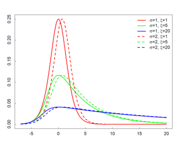
For all [math]\displaystyle{ \xi }[/math], the [math]\displaystyle{ \log \sigma }[/math] becomes the location parameter. See the right panel for the pdf when the shape [math]\displaystyle{ \xi }[/math] is positive.

The exGPD has finite moments of all orders for all [math]\displaystyle{ \sigma\gt 0 }[/math] and [math]\displaystyle{ -\infty\lt \xi \lt \infty }[/math].

The variance of the [math]\displaystyle{ exGPD(\sigma,\xi) }[/math] as a function of [math]\displaystyle{ \xi }[/math]. Note that the variance only depends on [math]\displaystyle{ \xi }[/math]. The red dotted line represents the variance evaluated at [math]\displaystyle{ \xi=0 }[/math], that is, [math]\displaystyle{ \psi'(1) = \pi^2/6 }[/math].

The moment-generating function of [math]\displaystyle{ Y \sim exGPD(\sigma,\xi) }[/math] is

[math]\displaystyle{ M_Y(s) = E[e^{sY}] = \begin{cases} -\frac{1}{\xi}\bigg(-\frac{\sigma}{\xi}\bigg)^{s} B(s+1, -1/\xi) \,\,\,\,\,\,\,\,\,\,\,\, \text{for } s \in (-1, \infty), \xi \lt 0 , \\ \frac{1}{\xi}\bigg(\frac{\sigma}{\xi}\bigg)^{s} B(s+1, 1/\xi - s) \,\,\,\,\,\, \,\,\,\,\,\,\,\,\,\,\, \text{for } s \in (-1, 1/\xi), \xi \gt 0 , \\ \sigma^{s} \Gamma(1+s) \,\,\,\,\,\,\,\,\,\,\,\,\,\,\,\,\,\,\,\,\,\,\,\,\,\, \,\,\,\,\,\,\,\,\,\,\,\,\,\,\,\,\,\,\,\,\,\,\,\,\,\,\,\, \text{for } s \in (-1, \infty), \xi = 0, \end{cases} }[/math]

where [math]\displaystyle{ B(a,b) }[/math] and [math]\displaystyle{ \Gamma (a) }[/math] denote the beta function and gamma function, respectively.

The expected value of [math]\displaystyle{ Y }[/math] [math]\displaystyle{ \sim }[/math] [math]\displaystyle{ exGPD }[/math] [math]\displaystyle{ ( }[/math][math]\displaystyle{ \sigma }[/math], [math]\displaystyle{ \xi }[/math] [math]\displaystyle{ ) }[/math] depends on the scale [math]\displaystyle{ \sigma }[/math] and shape [math]\displaystyle{ \xi }[/math] parameters, while the [math]\displaystyle{ \xi }[/math] participates through the digamma function:

[math]\displaystyle{ E[Y] = \begin{cases} \log\ \bigg(-\frac{\sigma}{\xi} \bigg)+ \psi(1) - \psi(-1/\xi+1) \,\,\,\,\,\,\,\,\,\,\,\, \,\, \text{for }\xi \lt 0 , \\ \log\ \bigg(\frac{\sigma}{\xi} \bigg)+ \psi(1) - \psi(1/\xi) \,\,\,\,\,\,\,\,\,\,\,\, \,\,\, \,\,\, \,\,\, \,\,\, \,\,\, \,\,\,\,\,\, \,\,\, \text{for }\xi \gt 0 , \\ \log \sigma + \psi(1) \,\,\,\,\,\,\,\,\,\,\,\,\,\,\,\,\,\,\,\,\,\,\,\,\,\, \,\,\, \,\,\, \,\,\, \,\,\,\,\,\,\,\,\,\,\,\,\,\,\,\,\,\,\,\,\,\,\,\,\,\,\, \,\,\, \,\,\,\,\,\,\, \text{for }\xi = 0. \end{cases} }[/math]

Note that for a fixed value for the [math]\displaystyle{ \xi \in (-\infty,\infty) }[/math], the [math]\displaystyle{ \log\ \sigma }[/math] plays as the location parameter under the exponentiated generalized Pareto distribution.

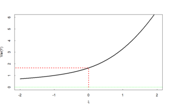
The variance of [math]\displaystyle{ Y }[/math] [math]\displaystyle{ \sim }[/math] [math]\displaystyle{ exGPD }[/math] [math]\displaystyle{ ( }[/math][math]\displaystyle{ \sigma }[/math], [math]\displaystyle{ \xi }[/math] [math]\displaystyle{ ) }[/math] depends on the shape parameter [math]\displaystyle{ \xi }[/math] only through the polygamma function of order 1 (also called the trigamma function):

[math]\displaystyle{ Var[Y] = \begin{cases} \psi'(1) - \psi'(-1/\xi +1) \,\,\,\,\,\,\,\,\,\,\,\, \, \text{for }\xi \lt 0 , \\ \psi'(1) + \psi'(1/\xi) \,\,\,\,\,\,\,\,\,\,\,\,\,\,\,\,\,\,\,\,\,\,\,\,\,\,\,\, \text{for }\xi \gt 0 , \\ \psi'(1) \,\,\,\,\,\,\,\,\,\,\,\,\,\,\,\,\,\,\,\,\,\,\,\,\,\,\,\,\,\,\,\,\,\,\,\,\,\,\,\,\,\,\,\,\,\,\,\,\,\, \,\,\,\,\,\text{for }\xi = 0. \end{cases} }[/math]

See the right panel for the variance as a function of [math]\displaystyle{ \xi }[/math]. Note that [math]\displaystyle{ \psi'(1) = \pi^2/6 \approx 1.644934 }[/math].

Note that the roles of the scale parameter [math]\displaystyle{ \sigma }[/math] and the shape parameter [math]\displaystyle{ \xi }[/math] under [math]\displaystyle{ Y \sim exGPD(\sigma, \xi) }[/math] are separably interpretable, which may lead to a robust efficient estimation for the [math]\displaystyle{ \xi }[/math] than using the [math]\displaystyle{ X \sim GPD(\sigma, \xi) }[/math] [2]. The roles of the two parameters are associated each other under [math]\displaystyle{ X \sim GPD(\mu=0,\sigma, \xi) }[/math] (at least up to the second central moment); see the formula of variance [math]\displaystyle{ Var(X) }[/math] wherein both parameters are participated.

The Hill's estimator

Assume that [math]\displaystyle{ X_{1:n} = (X_1, \cdots, X_n) }[/math] are [math]\displaystyle{ n }[/math] observations (not need to be i.i.d.) from an unknown heavy-tailed distribution [math]\displaystyle{ F }[/math] such that its tail distribution is regularly varying with the tail-index [math]\displaystyle{ 1/\xi }[/math] (hence, the corresponding shape parameter is [math]\displaystyle{ \xi }[/math]). To be specific, the tail distribution is described as

[math]\displaystyle{ \bar{F}(x) = 1 - F(x) = L(x) \cdot x^{-1/\xi}, \,\,\,\,\,\text{for some }\xi\gt 0,\,\,\text{where } L \text{ is a slowly varying function.} }[/math]

It is of a particular interest in the extreme value theory to estimate the shape parameter [math]\displaystyle{ \xi }[/math], especially when [math]\displaystyle{ \xi }[/math] is positive (so called the heavy-tailed distribution).

Let [math]\displaystyle{ F_u }[/math] be their conditional excess distribution function. Pickands–Balkema–de Haan theorem (Pickands, 1975; Balkema and de Haan, 1974) states that for a large class of underlying distribution functions [math]\displaystyle{ F }[/math], and large [math]\displaystyle{ u }[/math], [math]\displaystyle{ F_u }[/math] is well approximated by the generalized Pareto distribution (GPD), which motivated Peak Over Threshold (POT) methods to estimate [math]\displaystyle{ \xi }[/math]: the GPD plays the key role in POT approach.

A renowned estimator using the POT methodology is the Hill's estimator. Technical formulation of the Hill's estimator is as follows. For [math]\displaystyle{ 1\leq i \leq n }[/math], write [math]\displaystyle{ X_{(i)} }[/math] for the [math]\displaystyle{ i }[/math]-th largest value of [math]\displaystyle{ X_1, \cdots, X_n }[/math]. Then, with this notation, the Hill's estimator (see page 190 of Reference 5 by Embrechts et al [3]) based on the [math]\displaystyle{ k }[/math] upper order statistics is defined as

[math]\displaystyle{ \widehat{\xi}_{k}^{\text{Hill}} = \widehat{\xi}_{k}^{\text{Hill}}(X_{1:n}) = \frac{1}{k-1} \sum_{j=1}^{k-1} \log \bigg(\frac{X_{(j)}}{X_{(k)}} \bigg), \,\,\,\,\,\,\,\, \text{for } 2 \leq k \leq n. }[/math]

In practice, the Hill estimator is used as follows. First, calculate the estimator [math]\displaystyle{ \widehat{\xi}_{k}^{\text{Hill}} }[/math] at each integer [math]\displaystyle{ k \in \{ 2, \cdots, n\} }[/math], and then plot the ordered pairs [math]\displaystyle{ \{(k,\widehat{\xi}_{k}^{\text{Hill}})\}_{k=2}^{n} }[/math]. Then, select from the set of Hill estimators [math]\displaystyle{ \{\widehat{\xi}_{k}^{\text{Hill}}\}_{k=2}^{n} }[/math] which are roughly constant with respect to [math]\displaystyle{ k }[/math]: these stable values are regarded as reasonable estimates for the shape parameter [math]\displaystyle{ \xi }[/math]. If [math]\displaystyle{ X_1, \cdots, X_n }[/math] are i.i.d., then the Hill's estimator is a consistent estimator for the shape parameter [math]\displaystyle{ \xi }[/math] [4].

Note that the Hill estimator [math]\displaystyle{ \widehat{\xi}_{k}^{\text{Hill}} }[/math] makes a use of the log-transformation for the observations [math]\displaystyle{ X_{1:n} = (X_1, \cdots, X_n) }[/math]. (The Pickand's estimator [math]\displaystyle{ \widehat{\xi}_{k}^{\text{Pickand}} }[/math] also employed the log-transformation, but in a slightly different way [5].)

See also

• Burr distribution
• Pareto distribution
• Generalized extreme value distribution
• Exponentiated generalized Pareto distribution
• Pickands–Balkema–de Haan theorem

Further reading

• Pickands, James (1975). "Statistical inference using extreme order statistics". Annals of Statistics 3 s: 119–131. doi:10.1214/aos/1176343003. https://projecteuclid.org/journals/annals-of-statistics/volume-3/issue-1/Statistical-Inference-Using-Extreme-Order-Statistics/10.1214/aos/1176343003.pdf. 
• Balkema, A.; De Haan, Laurens (1974). "Residual life time at great age". Annals of Probability 2 (5): 792–804. doi:10.1214/aop/1176996548. 
• Lee, Seyoon; Kim, J.H.K. (2018). "Exponentiated generalized Pareto distribution:Properties and applications towards extreme value theory". Communications in Statistics - Theory and Methods 48 (8): 1–25. doi:10.1080/03610926.2018.1441418. 
• N. L. Johnson; S. Kotz; N. Balakrishnan (1994). Continuous Univariate Distributions Volume 1, second edition. New York: Wiley. ISBN 978-0-471-58495-7.  Chapter 20, Section 12: Generalized Pareto Distributions.
• Barry C. Arnold (2011). "Chapter 7: Pareto and Generalized Pareto Distributions". in Duangkamon Chotikapanich. Modeling Distributions and Lorenz Curves. New York: Springer. ISBN 9780387727967. https://books.google.com/books?id=fUJZZLj1kbwC&pg=PA119. 
• Arnold, B. C.; Laguna, L. (1977). On generalized Pareto distributions with applications to income data. Ames, Iowa: Iowa State University, Department of Economics. 

External links

• Mathworks: Generalized Pareto distribution

References

- ↑ Coles, Stuart (2001-12-12). An Introduction to Statistical Modeling of Extreme Values. Springer. p. 75. ISBN 9781852334598. https://books.google.com/books?id=2nugUEaKqFEC.
- ↑ Dargahi-Noubary, G. R. (1989). "On tail estimation: An improved method". Mathematical Geology 21 (8): 829–842. doi:10.1007/BF00894450. Bibcode: 1989MatGe..21..829D.
- ↑ Hosking, J. R. M.; Wallis, J. R. (1987). "Parameter and Quantile Estimation for the Generalized Pareto Distribution". Technometrics 29 (3): 339–349. doi:10.2307/1269343.
- ↑ Davison, A. C. (1984-09-30). "Modelling Excesses over High Thresholds, with an Application". in de Oliveira, J. Tiago. Statistical Extremes and Applications. Kluwer. p. 462. ISBN 9789027718044. https://books.google.com/books?id=6M03_6rm8-oC&pg=PA462.
- ↑ Embrechts, Paul; Klüppelberg, Claudia; Mikosch, Thomas (1997-01-01). Modelling extremal events for insurance and finance. Springer. p. 162. ISBN 9783540609315. https://books.google.com/books?id=BXOI2pICfJUC.
- ↑ 6.0 6.1 Jewson, Stephen; Sweeting, Trevor; Jewson, Lynne (2025-02-20). "Reducing reliability bias in assessments of extreme weather risk using calibrating priors" (in English). Advances in Statistical Climatology, Meteorology and Oceanography 11 (1): 1–22. doi:10.5194/ascmo-11-1-2025. ISSN 2364-3579. Bibcode: 2025ASCMO..11....1J. https://ascmo.copernicus.org/articles/11/1/2025/.
- ↑ https://cran.r-project.org/web/packages/fitdistcp/index.html
- ↑ https://cran.r-project.org/web/packages/Pareto/index.html