Asymmetric Laplace distribution
|
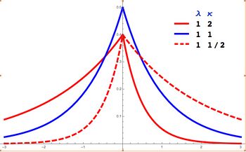
Probability density function  Asymmetric Laplace PDF with m = 0 in red. Note that the κ = 2 and 1/2 curves are mirror images. The κ = 1 curve in blue is the symmetric Laplace distribution. | |||
|
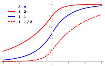
Cumulative distribution function  Asymmetric Laplace CDF with m = 0 in red. | |||
| Parameters |
[math]\displaystyle{ m }[/math] location (real) | ||
|---|---|---|---|
| Support | [math]\displaystyle{ x \in (-\infty; +\infty)\, }[/math] | ||
| (see article) | |||
| CDF | (see article) | ||
| Mean | [math]\displaystyle{ m+\frac{1-\kappa^2}{\lambda\kappa} }[/math] | ||
| Median |
[math]\displaystyle{ m+\frac{\kappa}{\lambda} \log\left(\frac{1+\kappa^2}{2\kappa^2}\right) }[/math] if [math]\displaystyle{ \kappa \gt 1 }[/math] [math]\displaystyle{ m-\frac{1}{\lambda \kappa} \log\left(\frac{1 + \kappa^2}{2} \right) }[/math] if [math]\displaystyle{ \kappa \lt 1 }[/math] | ||
| Variance | [math]\displaystyle{ \frac{1+\kappa^4}{\lambda^2\kappa^2} }[/math] | ||
| Skewness | [math]\displaystyle{ \frac{2 \left(1-\kappa ^6\right)}{\left(\kappa ^4+1\right)^{3/2}} }[/math] | ||
| Kurtosis | [math]\displaystyle{ \frac{6(1+\kappa^8)}{(1+\kappa^4)^2} }[/math] | ||
| Entropy | [math]\displaystyle{ \log\left(e\,\frac{1+\kappa^2}{\kappa\lambda}\right) }[/math] | ||
| CF | [math]\displaystyle{ \frac{ e^{i m t}}{(1+\frac{i t \kappa}{\lambda}) (1-\frac{i t}{\kappa\lambda})} }[/math] | ||
In probability theory and statistics, the asymmetric Laplace distribution (ALD) is a continuous probability distribution which is a generalization of the Laplace distribution. Just as the Laplace distribution consists of two exponential distributions of equal scale back-to-back about x = m, the asymmetric Laplace consists of two exponential distributions of unequal scale back to back about x = m, adjusted to assure continuity and normalization. The difference of two variates exponentially distributed with different means and rate parameters will be distributed according to the ALD. When the two rate parameters are equal, the difference will be distributed according to the Laplace distribution.
Characterization
Probability density function
A random variable has an asymmetric Laplace(m, λ, κ) distribution if its probability density function is[1][2]
- [math]\displaystyle{ f(x;m,\lambda,\kappa)=\left(\frac{\lambda}{\kappa+1/\kappa}\right)\, e^{-(x-m)\lambda\, s \kappa^s} }[/math]
where s=sgn(x-m), or alternatively:
- [math]\displaystyle{ f(x;m,\lambda,\kappa) = \frac{\lambda}{\kappa+1/\kappa} \begin{cases} \exp \left( (\lambda/\kappa)(x-m) \right) & \text{if }x \lt m \\[4pt] \exp ( -\lambda\kappa(x-m) ) & \text{if }x \geq m \end{cases} }[/math]
Here, m is a location parameter, λ > 0 is a scale parameter, and κ is an asymmetry parameter. When κ = 1, (x-m)s κs simplifies to |x-m| and the distribution simplifies to the Laplace distribution.
Cumulative distribution function
The cumulative distribution function is given by:
- [math]\displaystyle{ F(x;m,\lambda,\kappa) = \begin{cases} \frac{\kappa^2}{1+\kappa^2}\exp ((\lambda/\kappa)(x-m)) & \text{if }x \leq m \\[4pt] 1-\frac{1}{1+\kappa^2} \exp (-\lambda\kappa(x-m)) & \text{if }x \gt m \end{cases} }[/math]
Characteristic function
The ALD characteristic function is given by:
- [math]\displaystyle{ \varphi(t;m,\lambda,\kappa)=\frac{ e^{i m t}}{(1+\frac{i t \kappa}{\lambda}) (1-\frac{i t}{\kappa\lambda})} }[/math]
For m = 0, the ALD is a member of the family of geometric stable distributions with α = 2. It follows that if [math]\displaystyle{ \varphi_1 }[/math] and [math]\displaystyle{ \varphi_2 }[/math] are two distinct ALD characteristic functions with m = 0, then
- [math]\displaystyle{ \varphi=\frac{1}{1/\varphi_1+1/\varphi_2-1} }[/math]
is also an ALD characteristic function with location parameter [math]\displaystyle{ m=0 }[/math]. The new scale parameter λ obeys
- [math]\displaystyle{ \frac{1}{\lambda^2}=\frac{1}{\lambda_1^2}+\frac{1}{\lambda_2^2} }[/math]
and the new skewness parameter κ obeys:
- [math]\displaystyle{ \frac{\kappa^2-1}{\kappa\lambda}=\frac{\kappa_1^2-1}{\kappa_1\lambda_1}+\frac{\kappa_2^2-1}{\kappa_2\lambda_2} }[/math]
Moments, mean, variance, skewness
The n-th moment of the ALD about m is given by
- [math]\displaystyle{ E[(x-m)^n]=\frac{n!}{\lambda^n(\kappa+1/\kappa)}\,(\kappa^{-(n+1)}-(-\kappa)^{n+1}) }[/math]
From the binomial theorem, the n-th moment about zero (for m not zero) is then:
- [math]\displaystyle{ E[x^n]=\frac{\lambda\,m^{n+1}}{\kappa+1/\kappa}\,\left( \sum_{i=0}^n\frac{n!}{(n-i)!}\,\frac{1}{(m\lambda\kappa)^{i+1}} -\sum_{i=0}^n\frac{n!}{(n-i)!}\,\frac{1}{(-m\lambda/\kappa)^{i+1}} \right) }[/math]
- [math]\displaystyle{ = \frac{ \lambda \, m^{n+1}}{\kappa+1/\kappa} \left( e^{m \lambda\kappa} E_{-n}(m \lambda\kappa ) -e^{-m \lambda/\kappa } E_{-n}(-m \lambda /\kappa) \right) }[/math]
where [math]\displaystyle{ E_n( ) }[/math] is the generalized exponential integral function [math]\displaystyle{ E_n(x)=x^{n-1}\Gamma(1-n,x) }[/math]
The first moment about zero is the mean:
- [math]\displaystyle{ \mu=E[x]=m-\frac{\kappa-1/\kappa}{\lambda} }[/math]
The variance is:
- [math]\displaystyle{ \sigma^2=E[x^2]-\mu^2=\frac{1+\kappa^4}{\kappa^2\lambda^2} }[/math]
and the skewness is:
- [math]\displaystyle{ \frac{E[x^3]-3\mu\sigma^2-\mu^3}{\sigma^3}=\frac{2 \left(1-\kappa ^6\right)}{\left(\kappa ^4+1\right)^{3/2}} }[/math]
Generating asymmetric Laplace variates
Asymmetric Laplace variates (X) may be generated from a random variate U drawn from the uniform distribution in the interval (-κ,1/κ) by:
- [math]\displaystyle{ X=m-\frac{1}{\lambda\,s\kappa^s}\log(1-U\,s\kappa^S) }[/math]
where s=sgn(U).
They may also be generated as the difference of two exponential distributions. If X1 is drawn from exponential distribution with mean and rate (m1,λ/κ) and X2 is drawn from an exponential distribution with mean and rate (m2,λκ) then X1 - X2 is distributed according to the asymmetric Laplace distribution with parameters (m1-m2, λ, κ)
Entropy
The differential entropy of the ALD is
- [math]\displaystyle{ H=-\int_{-\infty}^\infty f_{AL}(x)\log(f_{AL}(x)) dx = 1-\log\left(\frac{\lambda}{\kappa+1/\kappa}\right) }[/math]
The ALD has the maximum entropy of all distributions with a fixed value (1/λ) of [math]\displaystyle{ (x-m)\,s\kappa^s }[/math] where [math]\displaystyle{ s=\sgn(x-m) }[/math].
Alternative parametrization
An alternative parametrization is made possible by the characteristic function:
[math]\displaystyle{ \varphi(t;\mu,\sigma,\beta)=\frac{ e^{i \mu t}}{1-i \beta \sigma t +\sigma^2 t^2} }[/math]
where [math]\displaystyle{ \mu }[/math] is a location parameter, [math]\displaystyle{ \sigma }[/math] is a scale parameter, [math]\displaystyle{ \beta }[/math] is an asymmetry parameter. This is specified in Section 2.6.1 and Section 3.1 of Lihn (2015). [3] Its probability density function is
- [math]\displaystyle{ f(x;\mu,\sigma,\beta) = \frac{1}{2 \sigma B_0} \begin{cases} \exp \left( \frac{x-\mu}{\sigma B^-} \right) & \text{if }x \lt \mu \\[4pt] \exp ( -\frac{x-\mu}{\sigma B^+} ) & \text{if }x \geq \mu \end{cases} }[/math]
where [math]\displaystyle{ B_0=\sqrt{1+\beta^2/4} }[/math] and [math]\displaystyle{ B^\pm=B_0\pm\beta/2 }[/math]. It follows that [math]\displaystyle{ B^+ B^- = 1,\P B^+ - B^- = \beta }[/math].
The n-th moment about [math]\displaystyle{ \mu }[/math] is given by
- [math]\displaystyle{ E[(x-\mu)^n]=\frac{\sigma^n n!}{2 B_0} ( (B^+)^{n+1} + (-1)^n (B^-)^{n+1} ) }[/math]
The mean about zero is:
[math]\displaystyle{ E[x]=\mu+\sigma \beta }[/math]
The variance is:
[math]\displaystyle{ E[x^2]-E[x]^2=\sigma^2 (2+\beta^2) }[/math]
The skewness is:
[math]\displaystyle{ \frac{2\beta (3+\beta^2)}{(2+\beta^2)^{3/2}} }[/math]
The excess kurtosis is:
[math]\displaystyle{ \frac{6 (2+4\beta^2+\beta^4)}{(2+\beta^2)^{2}} }[/math]
For small [math]\displaystyle{ \beta }[/math], the skewness is about [math]\displaystyle{ 3\beta/\sqrt{2} }[/math] . Thus [math]\displaystyle{ \beta }[/math] represents skewness in an almost direct way.
Alternative parameterization for Bayesian quantile regression
The Asymmetric Laplace distribution is commonly used with an alternative parameterization for performing quantile regression in a Bayesian inference context.[4] Under this approach, the [math]\displaystyle{ \kappa }[/math] parameter describing asymmetry is replaced with a [math]\displaystyle{ p }[/math] parameter indicating the percentile or quantile desired. Using this parameterization, the likelihood of the Asymmetric Laplace Distribution is equivalent to the loss function employed in quantile regression. With this alternative parameterization, the probability density function is defined as:
- [math]\displaystyle{ f(x;m,\lambda,p) = \frac{p(1-p)}{\lambda} \begin{cases} \exp \left( -((p-1)/\lambda)(x-m) \right) & \text{if }x \leq m \\[4pt] \exp ( -(p/\lambda)(x-m) ) & \text{if }x \gt m \end{cases} }[/math]
Where, m is a location parameter, λ > 0 is a scale parameter, and 0 < p < 1 is a percentile parameter.
The mean ([math]\displaystyle{ \mu }[/math]) and variance ([math]\displaystyle{ \sigma^2 }[/math]) are calculated as:
- [math]\displaystyle{ \mu=m+\frac{1-2p}{p(1-p)}\lambda }[/math]
- [math]\displaystyle{ \sigma^2=\frac{1-2p+2p^2}{p^2(1-p)^2}\lambda^2 }[/math]
The cumulative distribution function is given[5] by:
- [math]\displaystyle{ F(x;m,\lambda,p) = \begin{cases} p\exp (\frac{1-p}{\lambda}(x-m)) & \text{if }x \leq m \\[4pt] 1-(1-p) \exp (\frac{-p}{\lambda}(x-m)) & \text{if }x \gt m \end{cases} }[/math]
Applications
The asymmetric Laplace distribution has applications in finance and neuroscience. For the example in finance, S.G. Kou developed a model for financial instrument prices incorporating an asymmetric Laplace distribution to address problems of skewness, kurtosis and the volatility smile that often occur when using a normal distribution for pricing these instruments.[6] Another example is in neuroscience in which its convolution with normal distribution is considered as a model for brain stopping reaction times.[7]
References
- ↑ Kozubowski, Tomasz J.; Podgorski, Krzysztof (2000). "A Multivariate and Asymmetric Generalization of Laplace Distribution". Computational Statistics 15 (4): 531. doi:10.1007/PL00022717. https://www.researchgate.net/publication/256065510. Retrieved 2015-12-29.
- ↑ Jammalamadaka, S. Rao; Kozubowski, Tomasz J. (2004). "New Families of Wrapped Distributions for Modeling Skew Circular Data". Communications in Statistics – Theory and Methods 33 (9): 2059–2074. doi:10.1081/STA-200026570. http://www.pstat.ucsb.edu/faculty/jammalam/html/Some%20Publications/2004_WrappedSkewFamilies_Comm..pdf. Retrieved 2011-06-13.
- ↑ Lihn, Stephen H.-T. (2015). "The Special Elliptic Option Pricing Model and Volatility Smile". SSRN: 2707810. https://ssrn.com/abstract=2707810. Retrieved 2017-09-05.
- ↑ Yu, Keming; Moyeed, Rana A. (2001). "Bayesian quantile regression". Statistics & Probability Letters 54 (4): 437-447. doi:10.1016/S0167-7152(01)00124-9. https://www.sciencedirect.com/science/article/abs/pii/S0167715201001249. Retrieved 2022-01-09.
- ↑ Yu, Keming; Zhang, Jin (2005). "A Three-Parameter Asymmetric Laplace Distribution and Its Extension". Communications in Statistics - Theory and Methods 34 (9–10): 1867-1879. doi:10.1080/03610920500199018. https://www.tandfonline.com/doi/abs/10.1080/03610920500199018. Retrieved 2022-01-30.
- ↑ Kou, S.G. (August 8, 2002). "A Jump-Diffusion Model for Option Pricing". Management Science 48 (8): 1086–1101. doi:10.1287/mnsc.48.8.1086.166. https://www.jstor.org/stable/822677. Retrieved 2022-03-01.
- ↑ Soltanifar, M; Escobar, M; Dupuis, A; Chevrier, A; Schachar, R (2022). "The Asymmetric Laplace Gaussian (ALG) Distribution as the Descriptive Model for the Internal Proactive Inhibition in the Standard Stop Signal Task". Brain Sciences 12 (6): 730. doi:10.3390/brainsci12060730. PMID 35741615.
 |

