Hilbert curve
The Hilbert curve (also known as the Hilbert space-filling curve) is a continuous fractal space-filling curve first described by the German mathematician David Hilbert in 1891,[1] as a variant of the space-filling Peano curves discovered by Giuseppe Peano in 1890.[2]
Because it is space-filling, its Hausdorff dimension is 2 (precisely, its image is the unit square, whose dimension is 2 in any definition of dimension; its graph is a compact set homeomorphic to the closed unit interval, with Hausdorff dimension 2).
The Hilbert curve is constructed as a limit of piecewise linear curves. The length of the [math]\displaystyle{ n }[/math]th curve is [math]\displaystyle{ \textstyle 2^n - {1 \over 2^n} }[/math], i.e., the length grows exponentially with [math]\displaystyle{ n }[/math], even though each curve is contained in a square with area [math]\displaystyle{ 1 }[/math].
Images
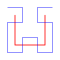
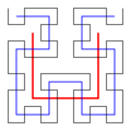
Variant, first three iterations[3]
Applications and mapping algorithms
Both the true Hilbert curve and its discrete approximations are useful because they give a mapping between 1D and 2D space that preserves locality fairly well.[4] This means that two data points which are close to each other in one-dimensional space are also close to each other after folding. The converse cannot always be true.
Because of this locality property, the Hilbert curve is widely used in computer science. For example, the range of IP addresses used by computers can be mapped into a picture using the Hilbert curve. Code to generate the image would map from 2D to 1D to find the color of each pixel, and the Hilbert curve is sometimes used because it keeps nearby IP addresses close to each other in the picture.[5] The locality property of the Hilbert curve has also been used to design algorithms for exploring regions with mobile robots.[6][7]
In an algorithm called Riemersma dithering, grayscale photograph can be converted to a dithered black-and-white image using thresholding, with the leftover amount from each pixel added to the next pixel along the Hilbert curve. Code to do this would map from 1D to 2D, and the Hilbert curve is sometimes used because it does not create the distracting patterns that would be visible to the eye if the order were simply left to right across each row of pixels.[8] Hilbert curves in higher dimensions are an instance of a generalization of Gray codes, and are sometimes used for similar purposes, for similar reasons. For multidimensional databases, Hilbert order has been proposed to be used instead of Z order because it has better locality-preserving behavior. For example, Hilbert curves have been used to compress and accelerate R-tree indexes[9] (see Hilbert R-tree). They have also been used to help compress data warehouses.[10][11]
The linear distance of any point along the curve can be converted to coordinates in n dimensions for a given n, and vice versa, using any of several standard mathematical techniques such as Skilling's method.[12][13]
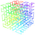
It is possible to implement Hilbert curves efficiently even when the data space does not form a square.[14] Moreover, there are several possible generalizations of Hilbert curves to higher dimensions.[15][16]
Representation as Lindenmayer system
The Hilbert Curve can be expressed by a rewrite system (L-system). File:Hilbert Curve - 6.webm
- Alphabet : A, B
- Constants : F + −
- Axiom : A
- Production rules:
- A → +BF−AFA−FB+
- B → −AF+BFB+FA−
Here, "F" means "draw forward", "+" means "turn left 90°", "-" means "turn right 90°" (see turtle graphics), and "A" and "B" are ignored during drawing.
Other implementations
Graphics Gems II[17] discusses Hilbert curve coherency, and provides implementation.
The Hilbert Curve is commonly used among rendering images or videos. Common programs such as Blender and Cinema 4D use the Hilbert Curve to trace the objects, and render the scene.[citation needed]
The slicer software used to convert 3D models into toolpaths for a 3D printer typically has the Hilbert curve as an option for an infill pattern.
See also
| Wikimedia Commons has media related to Hilbert curve. |
- Hilbert curve scheduling
- Hilbert R-tree
- Locality of reference
- Locality-sensitive hashing
- Moore curve
- Murray polygon
- Sierpiński curve
- List of fractals by Hausdorff dimension
Notes
- ↑ D. Hilbert: Über die stetige Abbildung einer Linie auf ein Flächenstück. Mathematische Annalen 38 (1891), 459–460.
- ↑ G.Peano: Sur une courbe, qui remplit toute une aire plane. Mathematische Annalen 36 (1890), 157–160.
- ↑ Bourges, Pascale. "Chapitre 1: fractales", Fractales et chaos. Accessed: 9 February 2019.
- ↑ Moon, B.; Jagadish, H.V.; Faloutsos, C.; Saltz, J.H. (2001), "Analysis of the clustering properties of the Hilbert space-filling curve", IEEE Transactions on Knowledge and Data Engineering 13 (1): 124–141, doi:10.1109/69.908985.
- ↑ "Mapping the whole internet with Hilbert curves". https://blog.benjojo.co.uk/post/scan-ping-the-internet-hilbert-curve.
- ↑ Spires, Shannon V.; Goldsmith, Steven Y. (1998), Drogoul, Alexis; Tambe, Milind; Fukuda, Toshio, eds., "Exhaustive geographic search with mobile robots along space-filling curves", Collective Robotics (Berlin, Heidelberg: Springer Berlin Heidelberg) 1456: pp. 1–12, doi:10.1007/bfb0033369, ISBN 978-3-540-64768-3, http://link.springer.com/10.1007/BFb0033369, retrieved 2023-08-14
- ↑ Sadat, Seyed Abbas; Wawerla, Jens; Vaughan, Richard (2015). "Fractal trajectories for online non-uniform aerial coverage". 2015 IEEE International Conference on Robotics and Automation (ICRA). pp. 2971–2976.
- ↑ Thiadmer Riemersma (1998-12-01). "A Balanced Dithering Technique". C/C++ User's Journal (Dr. Dobb's). https://www.drdobbs.com/a-balanced-dithering-technique/184403590.
- ↑ I. Kamel, C. Faloutsos, Hilbert R-tree: An improved R-tree using fractals, in: Proceedings of the 20th International Conference on Very Large Data Bases, Morgan Kaufmann Publishers Inc., San Francisco, CA, USA, 1994, pp. 500–509.
- ↑ Eavis, T.; Cueva, D. (2007). "A Hilbert Space Compression Architecture for Data Warehouse Environments". Data Warehousing and Knowledge Discovery. Lecture Notes in Computer Science. 4654. pp. 1–12. doi:10.1007/978-3-540-74553-2_1. ISBN 978-3-540-74552-5.
- ↑ Lemire, Daniel; Kaser, Owen (2011). "Reordering Columns for Smaller Indexes". Information Sciences 181 (12): 2550–2570. doi:10.1016/j.ins.2011.02.002.
- ↑ Programming The Hilbert Curve by John Skilling
- ↑ Grant Tebbin: Calculating Hilbert Curve Coordinates
- ↑ Hamilton, C. H.; Rau-Chaplin, A. (2007). "Compact Hilbert indices: Space-filling curves for domains with unequal side lengths". Information Processing Letters 105 (5): 155–163. doi:10.1016/j.ipl.2007.08.034.
- ↑ Alber, J.; Niedermeier, R. (2000). "On multidimensional curves with Hilbert property". Theory of Computing Systems 33 (4): 295–312. doi:10.1007/s002240010003.
- ↑ H. J. Haverkort, F. van Walderveen, Four-dimensional Hilbert curves for R-trees, in: Proceedings of the Eleventh Workshop on Algorithm Engineering and Experiments, 2009, pp. 63–73.
- ↑ Voorhies, Douglas: Space-Filling Curves and a Measure of Coherence, pp. 26–30, Graphics Gems II.
Further reading
- Warren Jr., Henry S. (2013). Hacker's Delight (2 ed.). Addison Wesley – Pearson Education, Inc.. ISBN 978-0-321-84268-8.
- McKenna, Douglas M. (2019). Hilbert Curves: Outside-In and Inside-Gone. Mathemaesthetics, Inc.. ISBN 978-1-7332188-0-1. http://www.mathemaesthetics.com/HilbertCurves.html.
External links
- Dynamic Hilbert curve with JSXGraph
- Three.js WebGL 3D Hilbert curve demo
- XKCD cartoon using the locality properties of the Hilbert curve to create a "map of the internet"
- Gcode generator for Hilbert curve
- Iterative algorithm for drawing Hilbert curve in JavaScript
- Algorithm 781: generating Hilbert's space-filling curve by recursion (ACM Digital Library)
 |


