Milstein method
In mathematics, the Milstein method is a technique for the approximate numerical solution of a stochastic differential equation. It is named after Grigori N. Milstein who first published it in 1974.[1][2]
Description
Consider the autonomous Itō stochastic differential equation: [math]\displaystyle{ \mathrm{d} X_t = a(X_t) \, \mathrm{d} t + b(X_t) \, \mathrm{d} W_t }[/math] with initial condition [math]\displaystyle{ X_{0} = x_{0} }[/math], where [math]\displaystyle{ W_{t} }[/math] stands for the Wiener process, and suppose that we wish to solve this SDE on some interval of time [math]\displaystyle{ [0,T] }[/math]. Then the Milstein approximation to the true solution [math]\displaystyle{ X }[/math] is the Markov chain [math]\displaystyle{ Y }[/math] defined as follows:
- partition the interval [math]\displaystyle{ [0,T] }[/math] into [math]\displaystyle{ N }[/math] equal subintervals of width [math]\displaystyle{ \Delta t\gt 0 }[/math]: [math]\displaystyle{ 0 = \tau_0 \lt \tau_1 \lt \dots \lt \tau_N = T\text{ with }\tau_n:=n\Delta t\text{ and }\Delta t = \frac{T}{N} }[/math]
- set [math]\displaystyle{ Y_0 = x_0; }[/math]
- recursively define [math]\displaystyle{ Y_n }[/math] for [math]\displaystyle{ 1 \leq n \leq N }[/math] by: [math]\displaystyle{ Y_{n + 1} = Y_n + a(Y_n) \Delta t + b(Y_n) \Delta W_n + \frac{1}{2} b(Y_n) b'(Y_n) \left( (\Delta W_n)^2 - \Delta t \right) }[/math] where [math]\displaystyle{ b' }[/math] denotes the derivative of [math]\displaystyle{ b(x) }[/math] with respect to [math]\displaystyle{ x }[/math] and: [math]\displaystyle{ \Delta W_n = W_{\tau_{n + 1}} - W_{\tau_n} }[/math] are independent and identically distributed normal random variables with expected value zero and variance [math]\displaystyle{ \Delta t }[/math]. Then [math]\displaystyle{ Y_n }[/math] will approximate [math]\displaystyle{ X_{\tau_n} }[/math] for [math]\displaystyle{ 0 \leq n \leq N }[/math], and increasing [math]\displaystyle{ N }[/math] will yield a better approximation.
Note that when [math]\displaystyle{ b'(Y_n) = 0 }[/math], i.e. the diffusion term does not depend on [math]\displaystyle{ X_{t} }[/math], this method is equivalent to the Euler–Maruyama method.
The Milstein scheme has both weak and strong order of convergence, [math]\displaystyle{ \Delta t }[/math], which is superior to the Euler–Maruyama method, which in turn has the same weak order of convergence, [math]\displaystyle{ \Delta t }[/math], but inferior strong order of convergence, [math]\displaystyle{ \sqrt{\Delta t} }[/math].[3]
Intuitive derivation
For this derivation, we will only look at geometric Brownian motion (GBM), the stochastic differential equation of which is given by: [math]\displaystyle{ \mathrm{d} X_t = \mu X \mathrm{d} t + \sigma X d W_t }[/math] with real constants [math]\displaystyle{ \mu }[/math] and [math]\displaystyle{ \sigma }[/math]. Using Itō's lemma we get: [math]\displaystyle{ \mathrm{d}\ln X_t= \left(\mu - \frac{1}{2} \sigma^2\right)\mathrm{d}t+\sigma\mathrm{d}W_t }[/math]
Thus, the solution to the GBM SDE is: [math]\displaystyle{ \begin{align} X_{t+\Delta t}&=X_t\exp\left\{\int_t^{t+\Delta t}\left(\mu-\frac{1}{2}\sigma^2\right)\mathrm{d}t+\int_t^{t+\Delta t}\sigma\mathrm{d}W_u\right\} \\ &\approx X_t\left(1+\mu\Delta t-\frac{1}{2} \sigma^2\Delta t+\sigma\Delta W_t+\frac{1}{2}\sigma^2(\Delta W_t)^2\right) \\ &= X_t + a(X_t)\Delta t+b(X_t)\Delta W_t+\frac{1}{2}b(X_t)b'(X_t)((\Delta W_t)^2-\Delta t) \end{align} }[/math] where [math]\displaystyle{ a(x) = \mu x, ~b(x) = \sigma x }[/math]
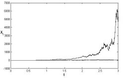
See numerical solution is presented above for three different trajectories.[4]
Computer implementation
The following Python code implements the Milstein method and uses it to solve the SDE describing the Geometric Brownian Motion defined by [math]\displaystyle{ \begin{cases} dY_t= \mu Y \, {\mathrm d}t + \sigma Y \, {\mathrm d}W_t \\ Y_0=Y_\text{init} \end{cases} }[/math]
# -*- coding: utf-8 -*-
# Milstein Method

import numpy as np
import matplotlib.pyplot as plt


class Model:
    """Stochastic model constants."""
    μ = 3
    σ = 1


def dW(Δt):
    """Random sample normal distribution."""
    return np.random.normal(loc=0.0, scale=np.sqrt(Δt))


def run_simulation():
    """ Return the result of one full simulation."""
    # One second and thousand grid points
    T_INIT = 0
    T_END = 1
    N = 1000 # Compute 1000 grid points
    DT = float(T_END - T_INIT) / N
    TS = np.arange(T_INIT, T_END + DT, DT)

    Y_INIT = 1

    # Vectors to fill
    ys = np.zeros(N + 1)
    ys[0] = Y_INIT
    for i in range(1, TS.size):
        t = (i - 1) * DT
        y = ys[i - 1]
        dw = dW(DT)

        # Sum up terms as in the Milstein method
        ys[i] = y + \
            Model.μ * y * DT + \
            Model.σ * y * dw + \
            (Model.σ**2 / 2) * y * (dw**2 - DT)

    return TS, ys


def plot_simulations(num_sims: int):
    """Plot several simulations in one image."""
    for _ in range(num_sims):
        plt.plot(*run_simulation())

    plt.xlabel("time (s)")
    plt.ylabel("y")
    plt.grid()
    plt.show()


if __name__ == "__main__":
    NUM_SIMS = 2
    plot_simulations(NUM_SIMS)
See also
References
- ↑ Mil'shtein, G. N. (1974). "Approximate integration of stochastic differential equations" (in ru). Teoriya Veroyatnostei i ee Primeneniya 19 (3): 583–588. http://www.mathnet.ru/php/archive.phtml?wshow=paper&jrnid=tvp&paperid=2929&option_lang=eng.
- ↑ Mil’shtein, G. N. (1975). "Approximate Integration of Stochastic Differential Equations". Theory of Probability & Its Applications 19 (3): 557–000. doi:10.1137/1119062.
- ↑ V. Mackevičius, Introduction to Stochastic Analysis, Wiley 2011
- ↑ Umberto Picchini, SDE Toolbox: simulation and estimation of stochastic differential equations with Matlab. http://sdetoolbox.sourceforge.net/
Further reading
- Kloeden, P.E., & Platen, E. (1999). Numerical Solution of Stochastic Differential Equations. Springer, Berlin. ISBN 3-540-54062-8.
 |


