Euler–Maruyama method
In Itô calculus, the Euler–Maruyama method (also called the Euler method) is a method for the approximate numerical solution of a stochastic differential equation (SDE). It is an extension of the Euler method for ordinary differential equations to stochastic differential equations. It is named after Leonhard Euler and Gisiro Maruyama. Unfortunately, the same generalization cannot be done for any arbitrary deterministic method.[1]
Consider the stochastic differential equation (see Itô calculus)
- [math]\displaystyle{ \mathrm{d} X_t = a(X_t, t) \, \mathrm{d} t + b(X_t, t) \, \mathrm{d} W_t, }[/math]
with initial condition X0 = x0, where Wt stands for the Wiener process, and suppose that we wish to solve this SDE on some interval of time [0, T]. Then the Euler–Maruyama approximation to the true solution X is the Markov chain Y defined as follows:
- partition the interval [0, T] into N equal subintervals of width [math]\displaystyle{ \Delta t\gt 0 }[/math]:
- [math]\displaystyle{ 0 = \tau_{0} \lt \tau_{1} \lt \cdots \lt \tau_{N} = T \text{ and } \Delta t = T/N; }[/math]
- set Y0 = x0
- recursively define Yn for 0 ≤ n ≤ N-1 by
- [math]\displaystyle{ \, Y_{n + 1} = Y_n + a(Y_n, \tau_n) \, \Delta t + b(Y_n, \tau_n) \, \Delta W_n, }[/math]
- where
- [math]\displaystyle{ \Delta W_n = W_{\tau_{n + 1}} - W_{\tau_n}. }[/math]
The random variables ΔWn are independent and identically distributed normal random variables with expected value zero and variance [math]\displaystyle{ \Delta t }[/math].
Example
Numerical simulation
An area that has benefited significantly from SDE is biology or more precisely mathematical biology. Here the number of publications on the use of stochastic model grew, as most of the models are nonlinear, demanding numerical schemes.
The graphic depicts a stochastic differential equation being solved using the Euler Scheme. The deterministic counterpart is shown as well.
Computer implementation
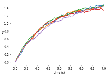
The following Python code implements the Euler–Maruyama method and uses it to solve the Ornstein–Uhlenbeck process defined by
- [math]\displaystyle{ dY_t=\theta \cdot (\mu-Y_t) \, {\mathrm d}t + \sigma \, {\mathrm d}W_t }[/math]
- [math]\displaystyle{ Y_0=Y_\mathrm{init}. }[/math]
The random numbers for [math]\displaystyle{ {\mathrm d}W_t }[/math] are generated using the NumPy mathematics package.
# -*- coding: utf-8 -*-
import numpy as np
import matplotlib.pyplot as plt


class Model:
    """Stochastic model constants."""
    THETA = 0.7
    MU = 1.5
    SIGMA = 0.06


def mu(y: float, _t: float) -> float:
    """Implement the Ornstein–Uhlenbeck mu."""
    return Model.THETA * (Model.MU - y)


def sigma(_y: float, _t: float) -> float:
    """Implement the Ornstein–Uhlenbeck sigma."""
    return Model.SIGMA


def dW(delta_t: float) -> float:
    """Sample a random number at each call."""
    return np.random.normal(loc=0.0, scale=np.sqrt(delta_t))


def run_simulation():
    """ Return the result of one full simulation."""
    T_INIT = 3
    T_END = 7
    N = 1000  # Compute at 1000 grid points
    DT = float(T_END - T_INIT) / N
    TS = np.arange(T_INIT, T_END + DT, DT)
    assert TS.size == N + 1

    Y_INIT = 0

    ys = np.zeros(TS.size)
    ys[0] = Y_INIT
    for i in range(1, TS.size):
        t = T_INIT + (i - 1) * DT
        y = ys[i - 1]
        ys[i] = y + mu(y, t) * DT + sigma(y, t) * dW(DT)

    return TS, ys


def plot_simulations(num_sims: int):
    """ Plot several simulations in one image."""
    for _ in range(num_sims):
        plt.plot(*run_simulation())

    plt.xlabel("time")
    plt.ylabel("y")
    plt.show()


if __name__ == "__main__":
    NUM_SIMS = 5
    plot_simulations(NUM_SIMS)
The following is simply the translation of the above code into the MATLAB (R2019b) programming language:
%% Initialization and Utility
close all;
clear all;

numSims = 5;            % display five runs
tBounds = [3 7];        % The bounds of t
N       = 1000;         % Compute at 1000 grid points
dt      = (tBounds(2) - tBounds(1)) / N ;
y_init  = 0;            % Initial y condition


% Initialize the probability distribution for our
% random variable with mean 0 and stdev of sqrt(dt)
pd = makedist('Normal',0,sqrt(dt));

c = [0.7, 1.5, 0.06];   % Theta, Mu, and Sigma, respectively

ts = linspace(tBounds(1), tBounds(2), N); % From t0-->t1 with N points
ys = zeros(1,N);     % 1xN Matrix of zeros

ys(1) = y_init;
%% Computing the Process
for j = 1:numSims
    for i = 2:numel(ts)
        t = tBounds(1) + (i-1) .* dt;
        y = ys(i-1);
        mu      = c(1) .* (c(2) - y);
        sigma   = c(3);
        dW      = random(pd);

        ys(i) = y + mu .* dt + sigma .* dW;
    end
    figure;
    hold on;
    plot(ts, ys, 'o')
end
See also
References
- ↑ Kloeden, P.E.; Platen, E. (1992). Numerical Solution of Stochastic Differential Equations. Springer, Berlin. ISBN 3-540-54062-8.
 |


