Gompertz distribution
|
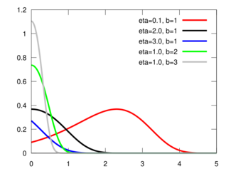
Probability density function  | |||
|
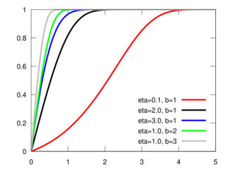
Cumulative distribution function  | |||
| Parameters | shape [math]\displaystyle{ \eta\gt 0\,\! }[/math], scale [math]\displaystyle{ b \gt 0\,\! }[/math] | ||
|---|---|---|---|
| Support | [math]\displaystyle{ x \in [0, \infty)\! }[/math] | ||
| [math]\displaystyle{ b\eta \exp\left(\eta + bx -\eta e^{bx} \right) }[/math] | |||
| CDF | [math]\displaystyle{ 1-\exp\left(-\eta\left(e^{bx}-1 \right)\right) }[/math] | ||
| Mean |
[math]\displaystyle{ (1/b)e^{\eta}\text{Ei}\left(-\eta\right) }[/math] [math]\displaystyle{ \text {where Ei}\left(z\right)=\int\limits_{-z}^{\infin}\left(e^{-v}/v\right)dv }[/math] | ||
| Median | [math]\displaystyle{ \left(1/b\right)\ln\left[\left(1/\eta\right)\ln\left(1/2\right)+1\right] }[/math] | ||
| Mode |
[math]\displaystyle{ =\left(1/b\right)\ln \left(1/\eta\right)\ }[/math] [math]\displaystyle{ \text {with }0 \lt \text {F}\left(x^*\right)\lt 1-e^{-1} = 0.632121, 0\lt \eta\lt 1 }[/math] [math]\displaystyle{ =0, \quad \eta \ge 1 }[/math] | ||
| Variance |
[math]\displaystyle{ \left(1/b\right)^2 e^{\eta}\{-2\eta { \ }_3\text {F}_3 \left(1,1,1;2,2,2;\eta\right)+\gamma^2 }[/math][math]\displaystyle{
+\left(\pi^2/6\right)+2\gamma\ln\left(\eta\right)+[\ln\left(\eta\right)]^2-e^{\eta}[\text{Ei}\left(-\eta \right)]^2\} }[/math] [math]\displaystyle{ \begin{align}\text{ where } &\gamma \text{ is the Euler constant: }\,\!\\ &\gamma=-\psi\left(1\right)=\text{0.577215... }\end{align} }[/math][math]\displaystyle{ \begin{align}\text { and } { }_3\text {F}_3&\left(1,1,1;2,2,2;-z\right)=\\&\sum_{k=0}^\infty\left[1/\left(k+1\right)^3\right]\left(-1\right)^k\left(z^k/k!\right)\end{align} }[/math] | ||
| MGF |
[math]\displaystyle{ \text{E}\left(e^{-t x}\right)=\eta e^{\eta}\text{E}_{t/b}\left(\eta\right) }[/math] [math]\displaystyle{ \text{with E}_{t/b}\left(\eta\right)=\int_1^\infin e^{-\eta v} v^{-t/b}dv,\ t\gt 0 }[/math] | ||
In probability and statistics, the Gompertz distribution is a continuous probability distribution, named after Benjamin Gompertz. The Gompertz distribution is often applied to describe the distribution of adult lifespans by demographers[1][2] and actuaries.[3][4] Related fields of science such as biology[5] and gerontology[6] also considered the Gompertz distribution for the analysis of survival. More recently, computer scientists have also started to model the failure rates of computer code by the Gompertz distribution.[7] In Marketing Science, it has been used as an individual-level simulation for customer lifetime value modeling.[8] In network theory, particularly the Erdős–Rényi model, the walk length of a random self-avoiding walk (SAW) is distributed according to the Gompertz distribution.[9]
Specification
Probability density function
The probability density function of the Gompertz distribution is:
- [math]\displaystyle{ f\left(x;\eta, b\right)=b\eta \exp\left(\eta + b x -\eta e^{bx} \right)\text{for }x \geq 0, \, }[/math]
where [math]\displaystyle{ b \gt 0\,\! }[/math] is the scale parameter and [math]\displaystyle{ \eta \gt 0\,\! }[/math] is the shape parameter of the Gompertz distribution. In the actuarial and biological sciences and in demography, the Gompertz distribution is parametrized slightly differently (Gompertz–Makeham law of mortality).
Cumulative distribution function
The cumulative distribution function of the Gompertz distribution is:
- [math]\displaystyle{ F\left(x;\eta, b\right)= 1-\exp\left(-\eta\left(e^{bx}-1 \right)\right) , }[/math]
where [math]\displaystyle{ \eta, b\gt 0, }[/math] and [math]\displaystyle{ x \geq 0 \, . }[/math]
Moment generating function
The moment generating function is:
- [math]\displaystyle{ \text{E}\left(e^{-t X}\right)=\eta e^{\eta}\text{E}_{t/b}\left(\eta\right) }[/math]
where
- [math]\displaystyle{ \text{E}_{t/b}\left(\eta\right)=\int_1^\infin e^{-\eta v} v^{-t/b}dv,\ t\gt 0. }[/math]
Properties
The Gompertz distribution is a flexible distribution that can be skewed to the right and to the left. Its hazard function [math]\displaystyle{ h(x)=\eta b e^{bx} }[/math] is a convex function of [math]\displaystyle{ F\left(x;\eta, b\right) }[/math]. The model can be fitted into the innovation-imitation paradigm with [math]\displaystyle{ p = \eta b }[/math] as the coefficient of innovation and [math]\displaystyle{ b }[/math] as the coefficient of imitation. When [math]\displaystyle{ t }[/math] becomes large, [math]\displaystyle{ z(t) }[/math] approaches [math]\displaystyle{ \infty }[/math]. The model can also belong to the propensity-to-adopt paradigm with [math]\displaystyle{ \eta }[/math] as the propensity to adopt and [math]\displaystyle{ b }[/math] as the overall appeal of the new offering.
Shapes
The Gompertz density function can take on different shapes depending on the values of the shape parameter [math]\displaystyle{ \eta\,\! }[/math]:
- When [math]\displaystyle{ \eta \geq 1,\, }[/math] the probability density function has its mode at 0.
- When [math]\displaystyle{ 0 \lt \eta \lt 1,\, }[/math] the probability density function has its mode at
- [math]\displaystyle{ x^*=\left(1/b\right)\ln \left(1/\eta\right)\text {with }0 \lt F\left(x^*\right)\lt 1-e^{-1} = 0.632121 }[/math]
Kullback-Leibler divergence
If [math]\displaystyle{ f_1 }[/math] and [math]\displaystyle{ f_2 }[/math] are the probability density functions of two Gompertz distributions, then their Kullback-Leibler divergence is given by
- [math]\displaystyle{ \begin{align} D_{KL} (f_1 \parallel f_2) & = \int_{0}^{\infty} f_1(x; b_1, \eta_1) \, \ln \frac{f_1(x; b_1, \eta_1)}{f_2(x; b_2, \eta_2)} dx \\ & = \ln \frac{e^{\eta_1} \, b_1 \, \eta_1}{e^{\eta_2} \, b_2 \, \eta_2} + e^{\eta_1} \left[ \left(\frac{b_2}{b_1} - 1 \right) \, \operatorname{Ei}(- \eta_1) + \frac{\eta_2}{\eta_1^{\frac{b_2}{b_1}}} \, \Gamma \left(\frac{b_2}{b_1}+1, \eta_1 \right) \right] - (\eta_1 + 1) \end{align} }[/math]
where [math]\displaystyle{ \operatorname{Ei}(\cdot) }[/math] denotes the exponential integral and [math]\displaystyle{ \Gamma(\cdot,\cdot) }[/math] is the upper incomplete gamma function.[10]
Related distributions
- If X is defined to be the result of sampling from a Gumbel distribution until a negative value Y is produced, and setting X=−Y, then X has a Gompertz distribution.
- The gamma distribution is a natural conjugate prior to a Gompertz likelihood with known scale parameter [math]\displaystyle{ b \,\!. }[/math][8]
- When [math]\displaystyle{ \eta\,\! }[/math] varies according to a gamma distribution with shape parameter [math]\displaystyle{ \alpha\,\! }[/math] and scale parameter [math]\displaystyle{ \beta\,\! }[/math] (mean = [math]\displaystyle{ \alpha/\beta\,\! }[/math]), the distribution of [math]\displaystyle{ x }[/math] is Gamma/Gompertz.[8]

- If [math]\displaystyle{ Y \sim \mathrm{Gompertz} }[/math], then [math]\displaystyle{ X = \exp(Y) \sim \mathrm{Weibull}^{-1} }[/math], and hence [math]\displaystyle{ \exp(-Y) \sim \mathrm{Weibull} }[/math].[12]
Applications
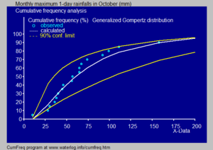
- In hydrology the Gompertz distribution is applied to extreme events such as annual maximum one-day rainfalls and river discharges. The blue picture illustrates an example of fitting the Gompertz distribution to ranked annually maximum one-day rainfalls showing also the 90% confidence belt based on the binomial distribution. The rainfall data are represented by plotting positions as part of the cumulative frequency analysis.
See also
- Gompertz-Makeham law of mortality
- Gompertz function
- Customer lifetime value
- Gamma Gompertz distribution
Notes
- ↑ Vaupel, James W. (1986). "How change in age-specific mortality affects life expectancy". Population Studies 40 (1): 147–157. doi:10.1080/0032472031000141896. PMID 11611920. http://pure.iiasa.ac.at/id/eprint/2683/1/WP-85-017.pdf.
- ↑ Preston, Samuel H.; Heuveline, Patrick; Guillot, Michel (2001). Demography:measuring and modeling population processes. Oxford: Blackwell.
- ↑ Benjamin, Bernard; Haycocks, H.W.; Pollard, J. (1980). The Analysis of Mortality and Other Actuarial Statistics. London: Heinemann.
- ↑ Willemse, W. J.; Koppelaar, H. (2000). "Knowledge elicitation of Gompertz' law of mortality". Scandinavian Actuarial Journal 2000 (2): 168–179. doi:10.1080/034612300750066845.
- ↑ Economos, A. (1982). "Rate of aging, rate of dying and the mechanism of mortality". Archives of Gerontology and Geriatrics 1 (1): 46–51. doi:10.1016/0167-4943(82)90003-6. PMID 6821142.
- ↑ Brown, K.; Forbes, W. (1974). "A mathematical model of aging processes". Journal of Gerontology 29 (1): 46–51. doi:10.1093/geronj/29.1.46. PMID 4809664.
- ↑ Ohishi, K.; Okamura, H.; Dohi, T. (2009). "Gompertz software reliability model: estimation algorithm and empirical validation". Journal of Systems and Software 82 (3): 535–543. doi:10.1016/j.jss.2008.11.840. http://ir.lib.hiroshima-u.ac.jp/00027703.
- ↑ 8.0 8.1 8.2 Bemmaor, Albert C.; Glady, Nicolas (2012). "Modeling Purchasing Behavior With Sudden 'Death': A Flexible Customer Lifetime Model". Management Science 58 (5): 1012–1021. doi:10.1287/mnsc.1110.1461.
- ↑ Tishby, Biham, Katzav (2016), The distribution of path lengths of self avoiding walks on Erdős-Rényi networks, arXiv:1603.06613.
- ↑ Bauckhage, C. (2014), Characterizations and Kullback-Leibler Divergence of Gompertz Distributions, arXiv:1402.3193.
- ↑ Calculator for probability distribution fitting [1]
- ↑ Kleiber, Christian; Kotz, Samuel (2003). Statistical Size Distributions in Economics and Actuarial Sciences. Wiley. p. 179. doi:10.1002/0471457175. ISBN 9780471150640. https://onlinelibrary.wiley.com/doi/book/10.1002/0471457175.
References
- Gompertz, B. (1825). "On the Nature of the Function Expressive of the Law of Human Mortality, and on a New Mode of Determining the Value of Life Contingencies". Philosophical Transactions of the Royal Society of London 115: 513–583. doi:10.1098/rstl.1825.0026. https://zenodo.org/record/1432356.
- Johnson, Norman L.; Kotz, Samuel; Balakrishnan, N. (1995). Continuous Univariate Distributions. 2 (2nd ed.). New York: John Wiley & Sons. pp. 25–26. ISBN 0-471-58494-0.
- Sheikh, A. K.; Boah, J. K.; Younas, M. (1989). "Truncated Extreme Value Model for Pipeline Reliability". Reliability Engineering and System Safety 25 (1): 1–14. doi:10.1016/0951-8320(89)90020-3.
 |

