Box counting

Box counting is a method of gathering data for analyzing complex patterns by breaking a dataset, object, image, etc. into smaller and smaller pieces, typically "box"-shaped, and analyzing the pieces at each smaller scale. The essence of the process has been compared to zooming in or out using optical or computer based methods to examine how observations of detail change with scale. In box counting, however, rather than changing the magnification or resolution of a lens, the investigator changes the size of the element used to inspect the object or pattern (see Figure 1). Computer based box counting algorithms have been applied to patterns in 1-, 2-, and 3-dimensional spaces.[1][2] The technique is usually implemented in software for use on patterns extracted from digital media, although the fundamental method can be used to investigate some patterns physically. The technique arose out of and is used in fractal analysis. It also has application in related fields such as lacunarity and multifractal analysis.[3][4]
The method
Theoretically, the intent of box counting is to quantify fractal scaling, but from a practical perspective this would require that the scaling be known ahead of time. This can be seen in Figure 1 where choosing boxes of the right relative sizes readily shows how the pattern repeats itself at smaller scales. In fractal analysis, however, the scaling factor is not always known ahead of time, so box counting algorithms attempt to find an optimized way of cutting a pattern up that will reveal the scaling factor. The fundamental method for doing this starts with a set of measuring elements—boxes—consisting of an arbitrary number, called here for convenience, of sizes or calibres, which we will call the set of s. Then these -sized boxes are applied to the pattern and counted. To do this, for each in , a measuring element that is typically a 2-dimensional square or 3-dimensional box with side length corresponding to is used to scan a pattern or data set (e.g., an image or object) according to a predetermined scanning plan to cover the relevant part of the data set, recording, i.e.,counting, for each step in the scan relevant features captured within the measuring element.[3][4]

The data
The relevant features gathered during box counting depend on the subject being investigated and the type of analysis being done. Two well-studied subjects of box counting, for instance, are binary (meaning having only two colours, usually black and white)[2] and gray-scale[5] digital images (i.e., jpegs, tiffs, etc.). Box counting is generally done on patterns extracted from such still images in which case the raw information recorded is typically based on features of pixels such as a predetermined colour value or range of colours or intensities. When box counting is done to determine a fractal dimension known as the box counting dimension, the information recorded is usually either yes or no as to whether or not the box contained any pixels of the predetermined colour or range (i.e., the number of boxes containing relevant pixels at each is counted). For other types of analysis, the data sought may be the number of pixels that fall within the measuring box,[4] the range or average values of colours or intensities, the spatial arrangement amongst pixels within each box, or properties such as average speed (e.g., from particle flow).[5][6][7][8]
Scan types
Every box counting algorithm has a scanning plan that describes how the data will be gathered, in essence, how the box will be moved over the space containing the pattern. A variety of scanning strategies has been used in box counting algorithms, where a few basic approaches have been modified in order to address issues such as sampling, analysis methods, etc.


Fixed grid scans
The traditional approach is to scan in a non-overlapping regular grid or lattice pattern.[3][4] To illustrate, Figure 2a shows the typical pattern used in software that calculates box counting dimensions from patterns extracted into binary digital images of contours such as the fractal contour illustrated in Figure 1 or the classic example of the coastline of Britain often used to explain the method of finding a box counting dimension. The strategy simulates repeatedly laying a square box as though it were part of a grid overlaid on the image, such that the box for each never overlaps where it has previously been (see Figure 4). This is done until the entire area of interest has been scanned using each and the relevant information has been recorded.[9] [10] When used to find a box counting dimension, the method is modified to find an optimal covering.
Sliding box scans
Another approach that has been used is a sliding box algorithm, in which each box is slid over the image overlapping the previous placement. Figure 2b illustrates the basic pattern of scanning using a sliding box. The fixed grid approach can be seen as a sliding box algorithm with the increments horizontally and vertically equal to . Sliding box algorithms are often used for analyzing textures in lacunarity analysis and have also been applied to multifractal analysis.[2][8][11][12][13]
Subsampling and local dimensions
Box counting may also be used to determine local variation as opposed to global measures describing an entire pattern. Local variation can be assessed after the data have been gathered and analyzed (e.g., some software colour codes areas according to the fractal dimension for each subsample), but a third approach to box counting is to move the box according to some feature related to the pixels of interest. In local connected dimension box counting algorithms, for instance, the box for each is centred on each pixel of interest, as illustrated in Figure 2c.[7]
Methodological considerations
The implementation of any box counting algorithm has to specify certain details such as how to determine the actual values in , including the minimum and maximum sizes to use and the method of incrementing between sizes. Many such details reflect practical matters such as the size of a digital image but also technical issues related to the specific analysis that will be performed on the data. Another issue that has received considerable attention is how to approximate the so-called "optimal covering" for determining box counting dimensions and assessing multifractal scaling.[5][14][15][16]
Edge effects
One known issue in this respect is deciding what constitutes the edge of the useful information in a digital image, as the limits employed in the box counting strategy can affect the data gathered.
Scaling box size
The algorithm has to specify the type of increment to use between box sizes (e.g., linear vs exponential), which can have a profound effect on the results of a scan.
Grid orientation
As Figure 4 illustrates, the overall positioning of the boxes also influences the results of a box count. One approach in this respect is to scan from multiple orientations and use averaged or optimized data.[17][18]
To address various methodological considerations, some software is written so users can specify many such details, and some includes methods such as smoothing the data after the fact to be more amenable to the type of analysis being done.[19]
See also
- Fractal analysis
- Fractal dimension
- Minkowski–Bouligand dimension
- Multifractal analysis
- Lacunarity
References
- ↑ Liu, Jing Z.; Zhang, Lu D.; Yue, Guang H. (2003). "Fractal Dimension in Human Cerebellum Measured by Magnetic Resonance Imaging". Biophysical Journal 85 (6): 4041–4046. doi:10.1016/S0006-3495(03)74817-6. PMID 14645092. Bibcode: 2003BpJ....85.4041L.
- ↑ 2.0 2.1 2.2 Smith, T. G.; Lange, G. D.; Marks, W. B. (1996). "Fractal methods and results in cellular morphology — dimensions, lacunarity and multifractals". Journal of Neuroscience Methods 69 (2): 123–136. doi:10.1016/S0165-0270(96)00080-5. PMID 8946315. https://zenodo.org/record/1259855.
- ↑ 3.0 3.1 3.2 Mandelbrot (1983). The Fractal Geometry of Nature. Henry Holt and Company. ISBN 978-0-7167-1186-5. https://archive.org/details/fractalgeometryo00beno.
- ↑ 4.0 4.1 4.2 4.3 Iannaccone, Khokha (1996). Fractal Geometry in Biological Systems. CRC Press. pp. 143. ISBN 978-0-8493-7636-8.
- ↑ 5.0 5.1 5.2 Li, J.; Du, Q.; Sun, C. (2009). "An improved box-counting method for image fractal dimension estimation". Pattern Recognition 42 (11): 2460–2469. doi:10.1016/j.patcog.2009.03.001. Bibcode: 2009PatRe..42.2460L.
- ↑ Karperien, Audrey; Jelinek, Herbert F.; Leandro, Jorge de Jesus Gomes; Soares, João V. B.; Cesar Jr, Roberto M.; Luckie, Alan (2008). "Automated detection of proliferative retinopathy in clinical practice". Clinical Ophthalmology 2 (1): 109–122. doi:10.2147/OPTH.S1579. PMID 19668394.
- ↑ 7.0 7.1 Landini, G.; Murray, P. I.; Misson, G. P. (1995). "Local connected fractal dimensions and lacunarity analyses of 60 degrees fluorescein angiograms". Investigative Ophthalmology & Visual Science 36 (13): 2749–2755. PMID 7499097.
- ↑ 8.0 8.1 Cheng, Qiuming (1997). "Multifractal Modeling and Lacunarity Analysis". Mathematical Geology 29 (7): 919–932. doi:10.1023/A:1022355723781.
- ↑ Popescu, D. P.; Flueraru, C.; Mao, Y.; Chang, S.; Sowa, M. G. (2010). "Signal attenuation and box-counting fractal analysis of optical coherence tomography images of arterial tissue". Biomedical Optics Express 1 (1): 268–277. doi:10.1364/boe.1.000268. PMID 21258464.
- ↑ King, R. D.; George, A. T.; Jeon, T.; Hynan, L. S.; Youn, T. S.; Kennedy, D. N.; Dickerson, B.; the Alzheimer’s Disease Neuroimaging Initiative (2009). "Characterization of Atrophic Changes in the Cerebral Cortex Using Fractal Dimensional Analysis". Brain Imaging and Behavior 3 (2): 154–166. doi:10.1007/s11682-008-9057-9. PMID 20740072.
- ↑ Plotnick, R. E.; Gardner, R. H.; Hargrove, W. W.; Prestegaard, K.; Perlmutter, M. (1996). "Lacunarity analysis: A general technique for the analysis of spatial patterns". Physical Review E 53 (5): 5461–5468. doi:10.1103/physreve.53.5461. PMID 9964879. Bibcode: 1996PhRvE..53.5461P.
- ↑ Plotnick, R. E.; Gardner, R. H.; O'Neill, R. V. (1993). "Lacunarity indices as measures of landscape texture". Landscape Ecology 8 (3): 201–211. doi:10.1007/BF00125351.
- ↑ McIntyre, N. E.; Wiens, J. A. (2000). "A novel use of the lacunarity index to discern landscape function". Landscape Ecology 15 (4): 313–321. doi:10.1023/A:1008148514268.
- ↑ Gorski, A. Z.; Skrzat, J. (2006). "Error estimation of the fractal dimension measurements of cranial sutures". Journal of Anatomy 208 (3): 353–359. doi:10.1111/j.1469-7580.2006.00529.x. PMID 16533317.
- ↑ Chhabra, A.; Jensen, R. V. (1989). "Direct determination of the f( alpha ) singularity spectrum". Physical Review Letters 62 (12): 1327–1330. doi:10.1103/PhysRevLett.62.1327. PMID 10039645. Bibcode: 1989PhRvL..62.1327C.
- ↑ Fernández, E.; Bolea, J. A.; Ortega, G.; Louis, E. (1999). "Are neurons multifractals?". Journal of Neuroscience Methods 89 (2): 151–157. doi:10.1016/s0165-0270(99)00066-7. PMID 10491946.
- ↑ Karperien (2004). Defining Microglial Morphology: Form, Function, and Fractal Dimension. Charles Sturt University, Australia.
- ↑ Schulze, M. M.; Hutchings, N.; Simpson, T. L. (2008). "The Use of Fractal Analysis and Photometry to Estimate the Accuracy of Bulbar Redness Grading Scales". Investigative Ophthalmology & Visual Science 49 (4): 1398–1406. doi:10.1167/iovs.07-1306. PMID 18385056.
- ↑ Karperien (2002), Box Counting, http://rsb.info.nih.gov/ij/plugins/fraclac/FLHelp/BoxCounting.htm#sampling
| Characteristics |    | |
|---|---|---|
| Iterated function system | ||
| Strange attractor | ||
| L-system | ||
| Escape-time fractals | ||
| Rendering techniques | ||
| Random fractals | ||
| People | ||
| Other | ||
 |  |
