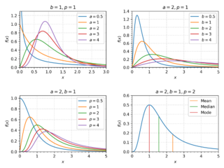
Dagum distribution
|
Probability density function  | |||
|
Cumulative distribution function  | |||
| Parameters |
shape shape scale | ||
|---|---|---|---|
| Support | |||
| CDF | |||
| Quantile | |||
| Mean |
[1] | ||
| Median | |||
| Mode | |||
| Variance | |||
| Entropy |
Where is the Harmonic numbers | ||
The Dagum distribution (or Mielke Beta-Kappa distribution) is a continuous probability distribution defined over positive real numbers. It is named after Camilo Dagum, who proposed it in a series of papers in the 1970s.[2][3] The Dagum distribution arose from several variants of a new model on the size distribution of personal income and is mostly associated with the study of income distribution. There is both a three-parameter specification (Type I) and a four-parameter specification (Type II) of the Dagum distribution; a summary of the genesis of this distribution can be found in "A Guide to the Dagum Distributions".[4] A general source on statistical size distributions often cited in work using the Dagum distribution is Statistical Size Distributions in Economics and Actuarial Sciences.[5]
Definition
The cumulative distribution function of the Dagum distribution (Type I) is given by
The corresponding probability density function is given by
The quantile function is given by
The Dagum distribution can be derived as a special case of the generalized Beta II (GB2) distribution (a generalization of the Beta prime distribution):
There is also an intimate relationship between the Dagum and Singh–Maddala / Burr distribution.
The cumulative distribution function of the Dagum (Type II) distribution adds a point mass at the origin and then follows a Dagum (Type I) distribution over the rest of the support (i.e. over the positive halfline)
The quantile function of the Dagum (Type II) distribution is
Use in economics
The Dagum distribution is often used to model income and wealth distribution. The relation between the Dagum Type I and the Gini coefficient is summarized in the formula below:[6]
where is the gamma function. Note that this value is independent from the scale-parameter, .
Derivation of the Gini coefficient for the Dagum distribution
|
|---|
|
The Gini coefficient for a continuous probability distribution takes the form: where is the CDF of the distribution and is the expected value. For the Dagum distribution, assuming , the formula for the Gini coefficient becomes: Defining the substitution leads to the simpler equation: And making the substitution further changes the Gini coefficient formula to: Each of the integral components is equivalent to the standard beta function, which may be written in terms of the gamma function: Then using this definition, and the fact that , the Gini coefficient may be written as: with the last term being the Gini coefficient for the Dagum distribution. |
Although the Dagum distribution is not the only three-parameter distribution used to model income distribution, one study found it to usually be a better fit than other three-parameter models.[7]
The Dagum distribution has been extended to model net wealth distribution, accounting for the observed frequencies of negative and null net wealth. This generalized model, known as the Dagum General Model of Net Wealth Distribution,[8] is a mixture model consisting of an atomic distribution at zero (representing economic units with no wealth) with two continuous distributions for negative and positive net wealth.
References
- ↑ Chotikapanich, Duangkamon et al. (2018). "Using the GB2 Income Distribution". Econometrics 6 (2): 21. doi:10.3390/econometrics6020021.
- ↑ Dagum, Camilo (1975). "A model of income distribution and the conditions of existence of moments of finite order". Bulletin of the International Statistical Institute 46 (Proceedings of the 40th Session of the ISI, Contributed Paper): 199–205.
- ↑ Dagum, Camilo (1977). "A new model of personal income distribution: Specification and estimation". Économie Appliquée 30: 413–437.
- ↑ Kleiber, Christian (2008). "A Guide to the Dagum Distributions". in Chotikapanich, Duangkamon. Modeling Income Distributions and Lorenz Curves. Economic Studies in Inequality, Social Exclusion and Well-Being. Springer. pp. 97–117. doi:10.1007/978-0-387-72796-7_6. ISBN 978-0-387-72756-1. https://edoc.unibas.ch/61230/1/20180305141821_5a9d439d76be5.pdf.
- ↑ Kleiber, Christian; Kotz, Samuel (2003). Statistical Size Distributions in Economics and Actuarial Sciences. Wiley. ISBN 0-471-15064-9.
- ↑ Kleiber, Christian (2007). "A Guide to the Dagum Distributions". Working Paper.
- ↑ Bandourian, Ripsy et al. (2002). "A Comparison of Parametric Models of Income Distribution Across Countries and Over Time". Luxembourg Income Study Working Paper No. 305.
- ↑ Dagum, Camilo (2006). "Wealth distribution models: analysis and applications" (in en). Statistica 66 (3): 235–268. doi:10.6092/issn.1973-2201/1243. ISSN 1973-2201. https://rivista-statistica.unibo.it/article/view/1243.
External links
- Camilo Dagum (1925 - 2005) : obituary
 |
