Datar–Mathews method for real option valuation

The Datar–Mathews Method (DM Method) is a method for real options valuation. The method provides an easy way to determine the real option value of a project simply by using the average of positive outcomes for the project. The method can be understood as an extension of the net present value (NPV) multi-scenario Monte Carlo model with an adjustment for risk aversion and economic decision-making. The method uses information that arises naturally in a standard discounted cash flow (DCF), or NPV, project financial valuation. It was created in 2000 by Vinay Datar, professor at Seattle University; and Scott H. Mathews, Technical Fellow at The Boeing Company.

Method

Fig. 1 Typical project cash flow with uncertainty

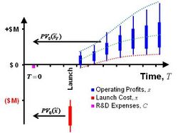
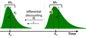
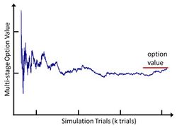
The mathematical equation for the DM Method is shown below. The method captures the real option value by discounting the distribution of operating profits at R, the market risk rate, and discounting the distribution of the discretionary investment at r, risk-free rate, before the expected payoff is calculated. The option value is then the expected value of the maximum of the difference between the two discounted distributions or zero. Fig. 1.

[math]\displaystyle{ C_0 = E \left[\max\left(\tilde S_Te^{-Rt}-\tilde X_Te^{-rt},0\right)\right] }[/math]

• [math]\displaystyle{ \tilde S_T }[/math] is a random variable representing the future benefits, or operating profits at time T. The present valuation of [math]\displaystyle{ \tilde S_T }[/math] uses R, a discount rate consistent with the risk level of [math]\displaystyle{ \tilde S_T, }[/math] [math]\displaystyle{ \tilde S_0=\tilde S_Te^{-RT}. }[/math] R is the required rate of return for participation in the target market, sometimes termed the hurdle rate.
• [math]\displaystyle{ \tilde X_T }[/math] is a random variable representing the strike price. The present valuation of [math]\displaystyle{ \tilde X_T }[/math] uses r, the rate consistent with the risk of capital investment of [math]\displaystyle{ \tilde X_T, }[/math] [math]\displaystyle{ \tilde X_0=\tilde X_Te^{-RT}. }[/math] In many generalized option applications, the risk-free discount rate is used. However other discount rates can be considered, such as the corporate bond rate, particularly when the application is an internal corporate product development project.
• [math]\displaystyle{ C_0 }[/math] is the real option value for a single stage project. The option value can be understood as the expected value of the difference of two present value distributions with an economically rational threshold limiting losses on a risk-adjusted basis. This value may also be expressed as a stochastic distribution.

The differential discount rate for R and r implicitly allows the DM Method to account for the underlying risk. If R > r, then the option will be risk-averse, typical for both financial and real options. If R < r, then the option will be risk-seeking. If R = r, then this is termed a risk-neutral option, and has parallels with NPV-type analyses with decision-making, such as decision trees. The DM Method gives the same results as the Black–Scholes and the binomial lattice option models, provided the same inputs and the discount methods are used. This non-traded real option value therefore is dependent on the risk perception of the evaluator toward a market asset relative to a privately held investment asset.

The DM Method is advantageous for use in real option applications because unlike some other option models it does not require a value for sigma (a measure of uncertainty) or for S₀ (the value of the project today), both of which are difficult to derive for new product development projects; see further under real options valuation. Finally, the DM Method uses real-world values of any distribution type, avoiding the requirement for conversion to risk-neutral values and the restriction of a lognormal distribution; see further under Monte Carlo methods for option pricing.

Extensions of the method for other real option valuations have been developed such as contract guarantee (put option), Multi-stage, Early Launch (American option), and others.

Implementation

The DM Method may be implemented using Monte-Carlo simulation, or in a simplified algebraic or other form (see the Range Option below).

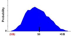
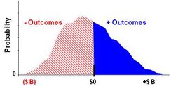
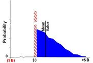
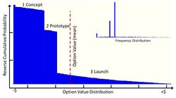
Using simulation, for each sample, the engine draws a random variable from both [math]\displaystyle{ \tilde S_T \text { and } \tilde X_T, }[/math] calculates their present values, and takes the difference. Fig. 2A. The difference value is compared to zero, the maximum of the two is determined, and the resulting value recorded by the simulation engine. Here, reflecting the optionality inherent in the project, a forecast of a net negative value outcome corresponds to an abandoned project, and has a zero value. Fig. 2B. The resulting values create a payoff distribution representing the economically rational set of plausible, discounted value forecasts of the project at time T₀.

Fig. 2A Net profit present-value distribution

Fig. 2B Rational decision distribution

Fig. 2C Payoff distribution and option value

When sufficient payoff values have been recorded, typically a few hundred, then the mean, or expected value, of the payoff distribution is calculated. Fig. 2C. The option value is the expected value, the first moment of all positive NPVs and zeros, of the payoff distribution.

A simple interpretation is:

[math]\displaystyle{ \text{Real option value} = \text{average} \left[\max\left(\text{operating profit}-\text{launch costs}\right),0)\right] }[/math]

where operating profit and launch costs are the appropriately discounted range of cash flows to time T₀.

The option value can also be understood as a distribution ([math]\displaystyle{ \tilde C_0 }[/math]) reflecting the uncertainty of the underlying variables.

DM Option Variations

Algebraic lognormal form

The DM real option can be considered a generalized form for option valuation. Its simulation produces a truncated present value distribution of which the mean value is interpreted to be the option value. With certain boundary conditions, the DM option can be reformulated algebraically as a conditional expectation of a lognormal distribution similar to the form and characteristics of a typical financial option, such as the European, single stage Black-Scholes financial option. This section illustrates the transformation of the DM real option to its algebraic lognormal form and its relationship to the Black-Scholes financial option formula. The process illuminates some of the more technical elements of the option formulation thereby providing further insight to the underlying concepts.

Fig. 3 Concept of conditional probability distribution and mean of tail

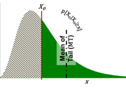
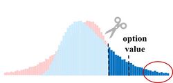
The lognormal form of the DM Method remains a simple concept based on the same computation procedures as the simulation form. It is the conditional expectation of the discounted projected future value outcome distribution, [math]\displaystyle{ \tilde S_T }[/math], less a predetermined purchase cost (strike price or launch cost), [math]\displaystyle{ \bar X_T }[/math], (modeled in this example as a scalar value) multiplied by the probability of that truncated distribution greater than a threshold—nominally 0. A conditional expectation is the expected value of the truncated distribution (mean of the tail), MT, computed with respect to its conditional probability distribution (Fig. 3).

Fig. 4 Time differentiated discounting appears to shift X relative to S

The option calculation procedure values the project investment (option purchase), C₀, at T₀. For the DM option the time differentiated discounting (R and r) results in an apparent shift of the projected value outcome distribution, [math]\displaystyle{ \tilde S }[/math], relative to the [math]\displaystyle{ \tilde X }[/math], or the scalar mean [math]\displaystyle{ \bar X }[/math] in the example shown in Fig. 4. This relative shift sets up the conditional expectation of the truncated distribution at T₀.

In a lognormal distribution for a project future value outcome, [math]\displaystyle{ \tilde S_T }[/math], both the mean, [math]\displaystyle{ \bar S_T }[/math], and standard deviation, [math]\displaystyle{ SD_T }[/math], must be specified. The standard deviation, [math]\displaystyle{ SD_T }[/math], of the distribution [math]\displaystyle{ \tilde S_T }[/math] is proportionately discounted along with the distribution, [math]\displaystyle{ SD_0 = SD_Te^{-RT}. }[/math]

The parameters of [math]\displaystyle{ \sigma \text{ and } \mu }[/math], of a lognormal at T₀ can be derived from the values [math]\displaystyle{ SD_0 \text{ and } S_0 }[/math] respectively, as:

[math]\displaystyle{ \sigma= \sqrt {\ln\left[1+\left(\tfrac{SD}{S}\right)^2\right] } \text { where } \tfrac {SD}{S}=\tfrac {SD_0}{S_0}= \tfrac {SD_T}{S_T} }[/math]

[math]\displaystyle{ \mu = \ln \left( \tfrac {S_0}{\sqrt {1 + \left( \tfrac {SD}{S} \right) ^2 }} \right)=\ln S_0 -0.5 \ln \left[ 1 + \left( \tfrac {SD}{S} \right) ^2 \right]=\ln S_0-0.5 \sigma^2. }[/math]

The conditional expectation of the discounted value outcome is the mean of the tail MT:

[math]\displaystyle{ E \left[ \tilde S \mid \tilde S \geq X \right]=S_0\left[\tfrac{N\left(\tfrac{\mu+\sigma^2-\ln X_0}{\sigma}\right)}{N\left(\tfrac{\mu-\ln X_0}{\sigma}\right)}\right]\text{ where }N(\cdot) }[/math] is the cumulative distribution function of the standard normal distribution (N(0,1)).

The probability of the project being in the money and launched (“exercised”) is [math]\displaystyle{ N\left(\tfrac{\mu-\ln X_0}{\sigma}\right). }[/math]

The project investment (option) value is:

[math]\displaystyle{ C_0=\left\{S_0\left[\tfrac{ N\left(\tfrac{\sigma^2+\mu-\ln X_0}{\sigma}\right)}{N\left(\tfrac{\mu-\ln X_0}{\sigma}\right)}\right]-X_0\right\} N \left(\tfrac{\mu-\ln X_0}{\sigma}\right). }[/math]

The involved lognormal mathematics can be burdensome and opaque for some business practices within a corporation. However, several simplifications can ease that burden and provide clarity without sacrificing the soundness of the option calculation. One simplification is the employment of the standard normal distribution, also known as the Z-distribution, which has a mean of 0 and a standard deviation of 1. It is common practice to convert a normal distribution to a standard normal and then use the standard normal table to find the value of probabilities.

Define as the standard normal variable: [math]\displaystyle{ Z=\tfrac{\left(\ln X_0-\mu\right)}{\sigma}. }[/math]

The conditional expectation of the discounted value outcome is:

[math]\displaystyle{ S_0\left[\tfrac{N\left(\tfrac{\mu+\sigma^2-\ln X_0}{\sigma}\right)}{N\left(\tfrac{\mu-\ln X_0}{\sigma}\right)}\right]=S_0\left[\tfrac{ N\left(\sigma-Z\right)}{ N\left(-Z\right)}\right]. }[/math]

Then probability of the project being in the money and launched (“exercised”) is: [math]\displaystyle{ N\left(\tfrac{\mu-\ln X_0}{\sigma}\right)=N\left(-Z\right). }[/math]

The Datar-Mathews lognormal option value simplifies to:

[math]\displaystyle{ C_\text{DM}=\left \{S_0\left[\tfrac{ N\left(\sigma-Z\right)}{ N\left(-Z\right)}\right]-X_0\right\} N\left(-Z\right)=S_0 N\left(\sigma-Z\right)-X_0 N\left(-Z\right). }[/math]

Transformation to the Black-Scholes Option

The Black–Scholes option formula (as well as the binomial lattice) is a special case of the simulated DM real option. With subtle, but notable differences, the logarithmic form of the DM Option can be algebraically transformed into The Black-Scholes option formula. The real option valuation is based on an approximation of the future value outcome distribution, which may be lognormal, at time T_T projected (discounted) to T₀. In contrast, the Black-Scholes is based on a lognormal distribution projected from historical asset returns to present time T₀. Analysis of these historical trends results in a calculation termed the volatility (finance) factor. For Black-Scholes (BS) the volatility factor is [math]\displaystyle{ \sigma_{BS}\sqrt T }[/math].

The following lognormal distribution with a standard deviation [math]\displaystyle{ \sigma }[/math] is replaced by the volatility factor [math]\displaystyle{ \sigma_{BS}\sqrt T }[/math].

[math]\displaystyle{ \left( \sigma -Z \right)=\sigma -\tfrac{\left(\ln X_0-\mu \right)}{\sigma}=\ln S_0 -0.5 \ln \left[ 1 + \left( \tfrac {SD}{S} \right) ^2 \right]=\tfrac{\left[ \ln\left( \tfrac{S_0}{X_T}\right)+\left( r+\tfrac{\sigma^2_\text {BS}}{2}\right) T\right]}{\left(\sigma_\text {BS} \sqrt T\right)}=d_1 \text { where } \ln X_T = \ln X_0 -rT }[/math]

[math]\displaystyle{ \left(-Z \right)= -\tfrac{\left(\ln X_0-\mu \right)}{\sigma}=\tfrac { \left [ \left (\ln S_0 -0.5 \sigma ^2 \right )-\ln X_0\right]}{\sigma}=\tfrac{\left[ \ln\left( \tfrac{S_0}{X_T}\right)+\left( r-\tfrac{\sigma^2_\text {BS}}{2}\right) T\right]}{\left(\sigma_\text {BS} \sqrt T\right)}=d_1-\sigma_\text {BS} \sqrt T=d_2 }[/math]

The Black-Scholes option value simplifies to its familiar form:

[math]\displaystyle{ C_\text{BS}=S N\left( d_1\right)-X_Te^{-rT} N\left( d_2\right) }[/math]

Fig 5. Left: Comparison of Black Scholes and Datar-Mathews frameworks. Right: Detail of tail of distribution at T₀.

The terms N(d₁) and N(d₂) are applied in the calculation of the Black–Scholes formula, and are expressions related to operations on lognormal distributions; see section "Interpretation" under Black–Scholes. Referring to Fig. 5 and using the lognormal form of the DM Option, it is possible to derive certain insights to the internal operation of an option:

[math]\displaystyle{ N\left(\sigma-Z\right)=N\left( d_1\right) }[/math]

[math]\displaystyle{ N\left(-Z\right)=N\left( d_2\right) }[/math]

N(-Z) or N(d₂) is a measure of the area of the tail of the distribution, MT (delineated by X₀), relative to that of the entire distribution, e.g. the probability of tail of the distribution, at time T₀. Fig. 5, Right. The true probability of expiring in-the-money in the real (“physical”) world is calculated at time T₀, the launch or strike date, measured by area of the tail of the distribution. N(σ-Z) or N(d₁) is the value of the option payoff relative to that of the asset. [math]\displaystyle{ N(d_1) = \left[MT \ x\ N(d_2)\right]/S_0, }[/math] where MT is the mean of the tail at time T₀.

Data patterns

Fig. 6 Option value (C₀) vs S₀/X₀ - UR constant

A simplified DM Method computation conforms to the same essential features—it is the discounted conditional expectation of the discounted projected future value outcome distribution, or [math]\displaystyle{ MT }[/math], less a discounted cost, [math]\displaystyle{ X_0 }[/math], multiplied by the probability of exercise, [math]\displaystyle{ N\left(-Z\right). }[/math] The value of the DM Method option can be understood as [math]\displaystyle{ C_0=\left(MT - X_0\right)\ x\ N\left(-Z\right). }[/math] This simplified formulation has strong parallels to an expected value calculation.

Businesses that collect historical data may be able to leverage the similarity of assumptions across related projects facilitating the calculation of option values. One resulting simplification is the Uncertainty Ratio, [math]\displaystyle{ \textstyle UR=(SD/S) }[/math], which can often be modeled as a constant for similar projects. UR is the degree of certainty by which the projected future cash flows can be estimated. UR is invariant of time [math]\displaystyle{ \textstyle\left(\tfrac{SD_T}{S_T}=\tfrac{SD_0}{S_0}\right) }[/math] with values typically between 0.35 and 1.0 for many multi-year business projects.

Applying this observation as a constant, K, to the above formulas results in a simpler formulation:

[math]\displaystyle{ \text {Define }K=\sigma =\sqrt \left [\ln (1+UR^2) \right ]\text {, and }\mu = \ln S_0-0.5\sigma ^2=\ln S_0-0.5K^2. }[/math]

[math]\displaystyle{ Z=\frac {(\ln X_0-\mu)}{\sigma}=\tfrac {\ln \left (\tfrac {X_0}{S_0}\right )}{K}+0.5K\text {, and } -Z=\tfrac {\ln \left (\tfrac {S_0}{X_0}\right )}{K}-0.5K. }[/math]

Variables	S0N(K-Z)-X0N(-Z)	S0(0.31S0/X0-0.10)
UR / K	0.6 / 0.55
S0/X0	1.0	1.0
Z	0.28
S0	$10.0M	$10.0M
C0	$2.18M	$2.10M
Difference		4%

[math]\displaystyle{ Z }[/math] is normally distributed and the values can be accessed in a table of standard normal variables. The resulting real option value can be derived simply on a hand-held calculator once K is determined:

[math]\displaystyle{ C_0=S_0 N\left (\sigma-Z\right )-X_0 N\left (-Z\right )= S_0 N\left (K-Z\right )-X_0 N\left (-Z\right ). }[/math]

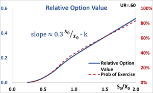
Assuming the UR is held constant, then the relative value of the option can simply be determined by the ratio of [math]\displaystyle{ S_0\text { and }X_0 }[/math], which is proportional to the probability of the project being in the money and launched (exercised). Then [math]\displaystyle{ \textstyle C_0 \approx S_0\ x\ \left [0.3 \ x\ (S_0/X_0) -k \right] . }[/math] (Fig. 6) A real option valuation is typically applied when the probability of exercise is approximately less than 50% [math]\displaystyle{ \left[(S_0/X_0) \lessapprox 1 \right]. }[/math] Businesses need apply their own data across similar projects to establish relevant parameter values.

Triangular form (Range Option)

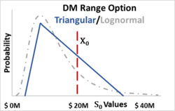
Given the difficulty in estimating the lognormal distribution mean and standard deviation of future returns, other distributions instead are more often applied for real options used in business decision making. The sampled distributions may take any form, although the triangular distribution is often used, as is typical for low data situations, followed by a uniform distribution (continuous) or a beta distribution. This approach is useful for early-stage estimates of project option value when there has not been sufficient time or resources to gather the necessary quantitative information required for a complete cash flow simulation, or in a portfolio of projects when simulation of all the projects is too computationally demanding. Regardless of the distribution chosen, the procedure remains the same for a real option valuation.

Fig. 7 Triangular conditional probability distribution

Innovation Project Quick Contingent Value Estimate

With most likely PV operating cash flow of $8.5M, but a 3-year capital cost of roughly $20M, the NPV of the important innovation project was deeply negative and the manager is considering abandoning it. Corporate sales analytics estimated with 95% certainty (double-sided 1-in-10 chance) the revenues could be as low as $4M or as high as $34M. (Fig. 8) Because of the large potential upside, the manager believes a small initial investment might resolve the project's downside uncertainties and reveal its potential value. Fig. 8 DM Range Option with triangular distribution. (Background: comparable lognormal distribution.) Using the DM Range Option as a guide, the manager calculated the expected contingent value of the project upside to be about $25M [≈ (2*$20M + $34M)/3]. Furthermore, there is a probability of one-in-four {25% ≈ ($34M - $20M)2 /[ ($34M - $4M)($34M-$8.5M)]} that the project revenues will be greater than $20M. With these calculations, the manager estimates the innovation project option value is $1.25M [= ($25M-$20M) * 25%]. Using this value, the manager justifies this initial investment (about 6% of the capital cost) into the project, sufficient to resolve some of the key uncertainties. The project can always be abandoned should the intermediate development results not measure up, but the investment losses will be minimized. (Later using corporate historical data patterns, an analyst converted the values from a three-point estimate to a DM Option calculation, and demonstrated that the result would differ by less than 10%.)

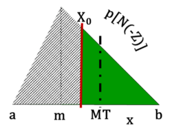
For a triangular distribution, sometimes referred to as three-point estimation, the mode value corresponds to the “most-likely” scenario, and the other two other scenarios, “pessimistic” and “optimistic”, represent plausible deviations from the most-likely scenario (often modeled as approximating a two-sided 1-out-of-10 likelihood or 95% confidence). This range of estimates results in the eponymous name for the option, the DM Range Option. The DM Range Option method is similar to the fuzzy method for real options. The following example (Fig. 7) uses a range of future estimated operating profits of a (pessimistic), b (optimistic) and m (mode or most-likely).

For [math]\displaystyle{ T_0 }[/math] discount a, b and m by [math]\displaystyle{ e^{-RT}\text { and } X_0=X_T e^{-rT}. }[/math]

The classic DM Method presumes that the strike price is represented by a random variable (distribution [math]\displaystyle{ \tilde X_0 }[/math]) with the option solution derived by simulation. Alternatively, without the burden of performing a simulation, applying the average or mean scalar value of the launch cost distribution [math]\displaystyle{ \bar X_0 }[/math] (strike price) results in a conservative estimate of DM Range Option value. If the launch cost is predetermined as a scalar value, then the DM Range Option value calculation is exact.

The expected value of the truncated triangular distribution (mean of the right tail), is [math]\displaystyle{ MT=\tfrac {\left (2X_0+b \right)}{3}. }[/math]

The probability of the project being in the money and launched is the proportional area of the truncated distribution relative to the complete triangular distribution. (See Fig. 17) This partial expectation is computed by the cumulative distribution function (CDF) given the probability distribution will be found at a value greater than or equal to X:

[math]\displaystyle{ P(X_0|X_0\ge x)=\frac{\left ( b-X_0 \right)^2}{\left [ \left ( b-a \right)\left(b-m\right ) \right ]}. }[/math]

The DM Range Option value, or project investment, is:

[math]\displaystyle{ C_0 = \left (MT - X_0 \right )\cdot P\left (X_0 \vert X_0 \ge x \right) =\left ( MT - X_0 \right )\cdot \left \{ \frac{\left ( b-X_0 \right)^2}{\left [ \left ( b-a \right)\left(b-m\right ) \right ]} \right \}. }[/math]

[math]\displaystyle{ \text {Note: }\mu =0.5*\ln (a+b)\text {, }\sigma=0.25*\ln (b/a)\text {, and } UR= \sqrt {e^ {\sigma^2} -1}. }[/math]

Use of a DM Range Option facilitates the application of real option valuation to future project investments. The DM Range Option provides an estimate of valuation that differs marginally with that of the DM Option algebraic lognormal distribution form. However, the projected future value outcome, S, of a project is rarely based on a lognormal distribution derived from historical asset returns, as is a financial option. Rather, the future value outcome, S, (as well as the strike price, X, and the standard deviation, SD), is more than likely a three-point estimation based on engineering and marketing parameters. Therefore, the ease of application of the DM Range Option is often justified by its expediency and is sufficient to estimate the conditional value of a future project.

Multi-stage (Compound) Option

Timothy Luehrman in an HBR article states: “In financial terms, a business strategy is much more like a series of options than a series of static cash flows or even decision trees. Executing a strategy almost always involves making a sequence of risky decisions.” A multi-stage business strategy valuation can be modeled as a sequence of staged contingent investment decisions structured as a series of DM single-stage options.

Fig. 9 Three-stage option value distribution.

In valuing a complex strategic opportunity, a multi-stage, or compound option, is a more accurate, but more mathematically demanding, approach than simpler calculations using decision tree model, influence diagrams, or lattice/binomial model approaches. Each stage is contingent on the execution or abandonment (gain/success or loss/failure) of the subsequent stage accounting for the investment cost of the preceding stages. The literature references several approaches to modeling a multi-stage option. A three-stage option (1 Proof of concept, 2 Prototype Development, 3 Launch/ Production) can be modeled as: [math]\displaystyle{ \begin{alignat}{2}C_0 = E \Bigl(& if \langle \left ( \tilde {S}_1e^{-Rt_0} \geq \tilde {X}_1e^{-rt_0} \right ), if \lbrace \left ( \tilde {S}_2e^{-Rt_0} \geq \tilde {X}_2e^{-rt_0} + \tilde {X}_1e^{-rt_0} \right ), \\ &\left [ max \left (\tilde {S}_3e^{-Rt_0} - \tilde {X}_3e^{-rt_0},0 \right ) - \tilde {X}_2e^{-rt_0} - \tilde {X}_1e^{-rt_0}\right ], - \tilde {X}_1e^{-rt_0} \rbrace ,0 \rangle \Bigr).\end{alignat} }[/math]

The valuation then occurs in reverse order conditioned on success or failure at each stage. The nominal value of this three-stage option is the mean of the multiple (typically several thousand k trials) simulated cash flows.

Fig. 10 Path dependency for selection of P* candidates.

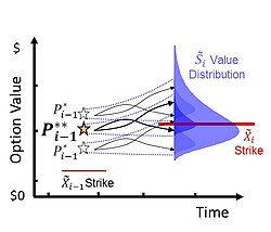
While the valuation of a multi-stage option is of technical interest, the principal focus of a project manager is the maximization of the probability of success and overall project value. The astute selection of project stage milestones can simultaneously achieve these goals while also providing project management clarity. Milestone set points are determined by specifying the option payoff for the end stage n value distribution, and backcasting. Prospective milestones, or value thresholds, for each stage i are designated [math]\displaystyle{ P_i^* }[/math] (pronounced ‘P-star’). Multiple simulated cash flows, projected from [math]\displaystyle{ \tilde {S}_0 }[/math], create a pattern of option value responses for each stage revealing prospective candidate milestones. The simulation evaluates the payoff option values [math]\displaystyle{ E \lbrace \left [ max \left ( \tilde {S}_ie^{-Rt_0} - \tilde {X}_ie^{-rt_0},0 \right ) - \tilde {X}_{i-1}e^{-rt_0}\right ] \geq P_i^*\rbrace. }[/math] A simulation of thousands of trials results in a valuation and ranking of a large sets of data pairs for each stage i: stage i option values mapped to candidate [math]\displaystyle{ P_i^* }[/math] values.

Fig. 11 Range of prospective milestones; optimal P** at vertex.

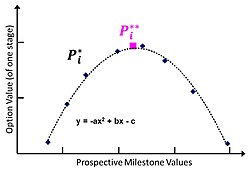
A parabolic distribution of data point pairs graphs the sorted range of stage i option values against prospective [math]\displaystyle{ P_i^* }[/math] milestone values. If selected [math]\displaystyle{ P_i^* }[/math] threshold is set too low, there are excessive failures to exercise, [math]\displaystyle{ \left ( \tilde {S}_ie^{-Rt_0} \lt P_i^*\right ) }[/math], and numerically the expected option value is reduced. Alternatively, if selected [math]\displaystyle{ P_i^* }[/math] threshold is set too high, then there are insufficient instances of successful exercises, and numerically the expected option value is reduced again. The optimal milestone [math]\displaystyle{ P_i^{**} }[/math] (‘P-double star’) value that emerges during simulation maximizes the overall project option value by balancing gains and losses.

Fig. 12 Emergent option value determined with P** candidates.

A three-stage option optimized for management by milestone and value maximization can be modeled as:

[math]\displaystyle{ \begin{alignat}{2}C_0=E \Bigl(& if \langle \left ( \tilde {S}_1e^{-Rt_0} \geq P_1^{**} \right ), if \lbrace \left ( \tilde {S}_2e^{-Rt_0} \geq P_2^{**} \right ), \\ &\left [ max \left (\tilde {S}_3e^{-Rt_0} - \tilde {X}_3e^{-rt_0},0 \right ) - \tilde {X}_2e^{-rt_0} - \tilde {X}_1e^{-rt_0}\right ], - \tilde {X}_1e^{-rt_0} \rbrace ,0 \rangle \Bigr). \end{alignat} }[/math]

Or, succinctly,

[math]\displaystyle{ C_0=E\left [max \left (\tilde {S}_ne^{-Rt_0} - \tilde {X}_ne^{-rt_0},0\right ) - \tilde {X}_{n-i}e^{-rt_0}\right ] \times \mathbb{P}\left ( \tilde {S}_1^{n-1}e^{-Rt_0}\geq P_1^{n-1 **}\right ). }[/math]

Note that typically [math]\displaystyle{ P_i^{**}\gg \tilde {X}_ie^{-rt_0}. }[/math] The insertion of these carefully determined conditional milestones increases the overall value of the nominal multi-stage option because each successive stage has been optimized to maximize the option value. By use of selected milestones, the project manager achieves the goals of increasing the probability of success and overall project value while also reducing the project managerial burden.

Demand Curve Integration

Fig. 13 Demand price and cost curves. Point of maximal profitability indicated by triangular markers.

Many early-stage projects find that the dominant unknown values are the first-order range estimates of the major components of operating profits: revenue and manufacturing cost of goods sold (COGS). In turn the uncertainty about revenue is driven by guesstimates of either market demand price or size. Market price and size can be estimated independently, though coupling them together in a market demand relationship is a better approach. COGS, the total of cost of product quantity to be sold, is the final component and trends according to an experience or learning curve cost relationship linked to market size. The interplay of these three market elements within a DM Real Options simulation, even with early-stage ranges, can reduce uncertainty for project planning by yielding reasonably narrowed target estimates for product pricing and production size that maximizes potential operating profits and improves option value.

Fig. 14 Left: A highly differentiated airfare market (MCO -- SFO) showing fare amounts paid by passengers (PAX). Right: Cumulative pareto ordering of data illustrating alignment with an inverse lognormal demand curve.

Fig. 15 A single instance example (simulation draw) of the three components that form the operating profits graph. The triangular markers indicate a maximum value for operating profit, delineating optimal price, units, and cost values. Yellow rows indicate optimal ranges.

A market price demand curve graphs the relationship of price to size, or quantity demanded. The law of demand states there is an inverse relationship between price and quantity demanded, or simply as the price decreases product quantity demanded will increase. A second curve, the manufacturing cost graph, models the learning curve effect illustrating the relationship between the quantity of goods produced and the efficiency gains of that production. Fig. 9. Mathematically, the learning curve takes the form of a power function.

A demand curve can be realistically modeled using an inverse lognormal distribution which convolves the market price distribution estimate with the market size range. A demand curve deftly models highly differentiated markets which through pricing distinguish selective product or service characteristics such as quality or grade, functional features, and availability, along with quantity sold. Examples are automobiles, shoes, smart phones, and computers. Airfare markets are highly differentiated where demand pricing and quantity sold are dependent on seasonality, day of week, time of day, routing, sale promotions, and seating or fare class. The airfare demand distribution pattern is well represented with an inverse lognormal distribution as shown in Fig. 10.

Curves for all the above components, market price, size, and COGS, can be simulated with variability to yield an optimal operating profit input for the real option calculation (Fig. 11). For example, the simulation results represented in Fig. 12. indicate ranges for price and unit quantity that potentially will maximize profitability. Extracted from these first-order range estimates, a selection of the peak (frequency) values identifies a significantly narrowed spread of promising estimates. Knowing these optimal value spreads substantially reduces uncertainty and provides a better, more targeted set of parameters from which to confidently base innovation development plans and option value.

Fig. 16 Optimal ranges to maximize profitability. Left: Price $56K - $62K. Right: Units 120K - 150K. Result is 85%+ improved estimate.

Comparison to other methods

The fuzzy pay-off method for real option valuation, created in 2009, provides another accessible approach to real option valuation. Though each use differing mathematical methods (Fuzzy: fuzzy logic; DM: numerical simulation and geometry) the underlying principal is strikingly similar: the likelihood of a positive payoff. Separately examining the two factors (possibility/probability, and positive payoff) demonstrates this similarity.

Fig. 17 Ratio of areas is proportional to the probability.

The possibility function for the fuzzy pay-off is [math]\displaystyle{ \tfrac{A(Pos)}{A(Pos)+A(Neg)} }[/math]. A simple interpretation is the proportionality ratio of the positive area of the fuzzy NPV over the total area of the fuzzy NPV. The probability of the project payoff for the DM Range Option is proportional to the area (CDF) of the positive distribution relative to the complete distribution. This is computed as [math]\displaystyle{ \tfrac{\left ( b-X_0 \right)^2}{\left [ \left ( b-a \right)\left(b-m\right ) \right ]}. }[/math] In each the ratios of the areas compute to the same possibility/probability value. The positive payoff of fuzzy pay-off simply is the mean of the positive area of the fuzzy NPV, or [math]\displaystyle{ E [A^+] }[/math]. Likewise, the positive payoff for the DM Range Option is the mean of the right tail (MT), or [math]\displaystyle{ \tfrac {\left (2X_0+b \right)}{3} }[/math] less the strike price [math]\displaystyle{ X_0 }[/math] This insight to the mechanics of the two methods illustrates not only their similarity but also their equivalency.

In a 2016 article in the Advances in Decision Sciences journal, researchers from the Lappeenranta University of Technology School of Business and Management compared the DM Method to the fuzzy pay-off method for real option valuation and noted that while the valuation results were similar, the fuzzy pay-off one was more robust in some conditions. In some comparative cases, the Datar-Mathews Method has a significant advantage in that it is easier to operate and connects NPV valuation and scenario analysis with Monte Carlo simulation (or geometry) technique thus greatly improving intuition in the usage of real options methods in managerial decision and explanation to third parties. Through its simulation interface, the Datar-Mathews Method easily accommodates multiple and sometimes correlated cash flow scenarios, including dynamic programming, typical of complex projects, such as aerospace, that are difficult to model using fuzzy sets.

DM Method and Prospect Theory

Real options are about objectively valuing innovation opportunities. Vexingly, these opportunities, evanescent and seemingly risky, are often comprehended subjectively. However, both the objective valuation mechanism and the subjective interpretation of results are often misunderstood leading to investment reluctance and potentially undervaluing opportunities.

The DM real option employs the objective valuation formula [math]\displaystyle{ C_0 = E [\max (...,{\color {red} 0)}], }[/math] where [math]\displaystyle{ \color {red} 0 }[/math] is the default threshold when it is economically rational to terminate (abandon) an opportunity event. If a simulation event (‘draw’) calculates a negative outcome (i.e., [math]\displaystyle{ [ \tilde S_T e^{-Rt} \leq \tilde X_T e^{-rt} ], }[/math] operating profits less than launch costs), then that event outcome should be rationally cut, or terminated, recording a [math]\displaystyle{ \color {red} 0 }[/math] residual. Only net positive economic outcomes [math]\displaystyle{ [ \tilde S_T e^{-Rt} \gt \tilde X_T e^{-rt} ] }[/math] are tallied. This operation leaves the misperception of ‘the odds being stacked’ favoring only positive outcomes seemingly resulting in an abnormally high valuation. However, the [math]\displaystyle{ E }[/math] of the formula [math]\displaystyle{ C_0 = E [\max (...,0)] }[/math] mathematically calculates the correct option value by adjusting these positive outcomes according to their likelihood, i.e., probability of a success (POS).

The actual DM formula is [math]\displaystyle{ C_0 = E [\max (...,{\color {red} ?})], }[/math] where the threshold [math]\displaystyle{ \color {red} ? }[/math] (‘floor’) can assume any value (or alternative formula) including the default [math]\displaystyle{ \color {red} 0 }[/math]. Using a threshold other than [math]\displaystyle{ \color {red} 0 }[/math] transforms the formula into a hurdle-weighted option variation. The result is no longer equivalent to the value of a financial option.

Fig. 18 Low probability, high value outcomes (red circle).

Much of the perceived high value of a real option valuation is disproportionately located in the far-right end of the tail of the simulation distribution, an area of low probability but high value outcomes. The option valuation reflects the potential opportunity value if the various outcome assumptions are validated. Targeted, incremental investments can validate these low probability assumptions. If not, replace the assumptions with proven ‘plausible’ elements, then recalculate the value based on new learnings.

The subjective undervaluation of real options partially can be explained by behavioral sciences. An innovation investor may perceive the initial investments to be potentially at a loss, particularly if the POS is low. Kahneman and Tversky's Prospect theory proclaims that losses are perceived to have an impact more than twice that of gains for the same value. The result is the loss averse investor will subjectively undervalue the opportunity, and therefore the investment, despite the objective and financially accurate real option valuation.

Regret aversion, another behavioral science observation, occurs when an unfounded decision is made to avoid regretting a future outcome. For example, a regret-averse investor decides to invest in a relatively ‘sure bet’ but smaller payoff opportunity relative to an alternative with a significantly higher but presumably uncertain payoff. The regret aversion phenomenon is closely aligned with uncertainty aversion (certainty bias), where the unknown aspects of the innovation opportunity (i.e., newness, lack of control) are rationalized as a hurdle to further investments. The consequences of loss- and regret-averse decision-making are parsimonious investments and underfunding (‘undervaluing’) of promising early-stage innovation opportunities.

A savvy investor can overcome the perceived mis-valuation of an option price. Loss aversion registers significantly high when the entire option value is interpreted as investment risk. This emotional response fails to consider that the initial early-stage investments are only a fraction of the entire option value, necessarily targeted to validate the most salient assumptions. Similarly regret aversion should not be misconceived as risk aversion because the exposure of small early-stage investments is usually not material. Instead, these initial investments carefully probe the opportunity's core value while providing a sense of control over an otherwise uncertain outcome. Regret is minimized by the realization that the opportunity development can be terminated if the assumption outcomes are not promising. The investment funds expended are prudently applied only to investigate a promising opportunity, and, in return, are enhanced by the acquired knowledge.

Since individuals are prone to cognitive biases, various intervention strategies are designed to reduce them including expert review along with bias andnaïve realism awareness. A phenomenon termed “bias blind spot” succinctly describes an individual's unconscious susceptibility to biases. This fundamental attribution error remains subconsciously hidden by an illusion of self-introspection, i.e., that we believe, falsely, we have access to our inner intentions or motivations. Biases may be post hoc rationalized away, but nonetheless impact decision-making. To counteract biases, it is insufficient simply be aware of their characteristics, but necessary also to become educated of one's own introspection illusion.

References

- ↑ Mathews, Scott; Datar, Vinay; Johnson, Blake (2007). "A Practical Method for Valuing Real Options: The Boeing Approach". Journal of Applied Corporate Finance 19 (2): 95–104. doi:10.1111/j.1745-6622.2007.00140.x.
- ↑ U.S. Patent No. 6,862,579 (issued March 1, 2005).
- ↑ Nugroho, Lukito Adi; McMillan, David (28 April 2017). "Real options valuation of franchise territorial exclusivity". Cogent Business & Management 4 (1): 4–5. doi:10.1080/23311975.2016.1262490.
- ↑ Barton, Kelsey; Lawryshyn, Yuri (2010-06-17). "Reconciling Real Option Models: An Approach to Incorporate Market and Private Uncertainties". Real Options: Theory Meets Practice - 14th Annual International Conference. Rome, Italy. http://realoptions.org/papers2010/106.pdf.
- ↑ Savolainen, Jyrki; Collan, Mikael; Luukka, Pasi (2016). "Combining System Dynamic Modeling and the Datar–Mathews Method for Analyzing Metal Mine Investments". Acta Universitatis Palackianae Olomucensis. Facultas Rerum Naturalium. Mathematica 55 (1): 95–110. ISSN 0231-9721.
- ↑ Datar, Vinay T. and Mathews, Scott H., 2004. European Real Options: An Intuitive Algorithm for the Black–Scholes Formula.
- ↑ Brigatti, E; Macias F.; Souza M.O.; Zubelli J.P. (2015). Aid, R. ed. A Hedged Monte Carlo Approach to Real Option Pricing. New York, NY: Springer. p. 7. doi:10.1007/978-1-4939-2733-3_10. ISBN 978-1-4939-2733-3.
- ↑ Business Engineering: A Practical Approach to Valuing High-Risk, High-Return Projects Using Real Options Tutorials in Operations Research 2007, Operations Research Tools and Applications: Glimpses of Future Technologies, p157–175
- ↑ Business Engineering: A Practical Approach to Valuing High-Risk, High-Return Projects Using Real Options INFORMS Annual Meeting, November 4–7, 2007
- ↑ Kozlova, Mariia (April 2015). Analyzing the Effects of the New Renewable Energy Policy in Russia on Investments into Wind, Solar and Small Hydro Power (Thesis). Lappeenranta University of Technology. pp. 62–66.
- ↑ Mathews, Scott H., 2009. Tutorial CIFER-T2 Boeing's method for valuing high-risk high-return technology projects using real options. IEEE Symposium on Computational Intelligence for Financial Engineering, 2009.
- ↑ Gyoshev, Stanley B.; Gombola, Michael (2012-12-04). "A Separating Equilibrium for Stock Repurchase Programs via PUT Options: Transforming a Mathematical Proof into Visual Form" (in en). SSRN Working Paper Series: 4, 17. doi:10.2139/ssrn.2185093. ISSN 1556-5068. https://ssrn.com/abstract=2185093.
- ↑ Luenberger, David (Autumn 1998). "The Two-Rate Method of Discounting". Department of Management Science & Engineering, Stanford University. http://www.investmentscience.com/Content/newsArticles/news3.html.
- ↑ Justin, Cedric Yves; Mavris, Dimitri N. (2011-09-20). "Option-Based Approach to Value Engine Maintenance Cost Guarantees and Engine Maintenance Contracts". 11th AIAA Aviation Technology, Integration, and Operations (ATIO) Conference. p. 7. doi:10.2514/6.2011-6839.
- ↑ Mathews, Scott (2010). "Valuing High-Risk High-Return technology Projects Using Real Options". in Bidgoli, Hossein. The Handbook of Technology Management: Core Concepts, Financial Tools and Techniques, Operations and Innovation Management. 1. Hoboken, NJ: Wiley. pp. 581–600. ISBN 978-0470249475.
- ↑ Hereafter, variables are assumed to be scaler unless otherwise specified as a distribution indicated by a tilde [math]\displaystyle{ \sim. }[/math]
- ↑ Collan, Mikael (2011). "Thoughts about Selected Models for the Valuation of Real Options". Acta Universitatis Palackianae Olomucensis. Facultas Rerum Naturalium. Mathematica 50 (2): 5–12. ISSN 0231-9721. http://dml.cz/dmlcz/141747.
- ↑ The Black-Scholes model classically assumed that a lognormal distribution most closely approximated the statistical distribution of an asset’s returns. This assumption conveniently simplified the mathematics of the option pricing formula and it remains a useful approximation. In reality security prices do not follow a strict stationary log-normal process. The value results using the Black–Scholes model differ slightly from real world financial option prices in part because of simplifying assumptions of the model.
- ↑ Variance of a lognormal distribution is [math]\displaystyle{ \sigma ^2 }[/math], and its standard deviation is [math]\displaystyle{ \sigma }[/math]. Variance of stock prices are assumed to follow a Wiener Process or geometric Brownian motion proportional to time [math]\displaystyle{ \sigma ^2 T }[/math] and its standard deviation (or volatility) is [math]\displaystyle{ \sigma \sqrt T }[/math]. The relationship of Black Scholes (BS) volatility (annualized) and the logarithmic standard deviation is then: [math]\displaystyle{ \sigma _{BS} \sqrt T =\sigma . }[/math] Alternatively, [math]\displaystyle{ \sigma _{BS} =\sqrt \tfrac { \ln \left [ 1+ \left ( \tfrac {SD} {S} \right ) ^2 \right ]} {T} }[/math] where S is the mean and SD is the standard deviation of the present value lognormal distribution.
- ↑ Houstecky, Petr. "Why Is Volatility Proportional to the Square Root of Time?". https://www.macroption.com/why-is-volatility-proportional-to-square-root-of-time/.
- ↑ Don Chance (2011). Derivation and Interpretation of the Black–Scholes Model .
- ↑ Care must be taken when [math]\displaystyle{ S_0 \ll X_0 }[/math] owing to the non-linearities of real option mathematics. When [math]\displaystyle{ S_0 \gg X_0 }[/math] then an NPV-style valuation may be undertaken.
- ↑ Alabi, Olabode (2010-04-30). Evaluation Method for Strategic Investments (Dissertation). University of Nebraska - Lincoln.
- ↑ Peters, Linda (September 2016). "Impact of Probability Distributions on Real Options Valuation". Journal of Infrastructure Systems 22 (3): 04016005. doi:10.1061/(ASCE)IS.1943-555X.0000289.
- ↑ Innovation Portfolio Architecture – Part 2: Attribute Selection and Valuation . Research-Technology Management Vol. 54, No. 5 September–October 2011
- ↑ Sadowsky, Jeffery R. (May 10, 2005). "The Value of Learning in the Product Development Stage: A Real Options Approach". SSRN: 9. doi:10.2139/ssrn.721597.
- ↑ Onkham, Wilawan (2013). A Real Option Dynamic Decision Framework for Operational Innovations (PhD). University of Central Florida. p. 44.
- ↑ Naedele, Martin; Chen, Hong-Mei; Kazman, Rick; Cai, Yuanfang; Xiao, Lu; Silva, Carlos V.A. (March 2015). "Manufacturing execution systems: A vision for managing software development". Journal of Systems and Software 101: 59–68. doi:10.1016/j.jss.2014.11.015.
- ↑ Patregnani, Giulia (2014-10-13). The Value of Synergies through the Real Options Lenses (Graduate Theses, MS in Finance and Strategic Management). Copenhagen School of Business. pp. 63–65. hdl:10417/4840.
- ↑ Mathews, Scott (September–October 2009). "Valuing Risky Projects with Real Options" (in en). Research Technology Management 52 (5): 32–41. doi:10.1080/08956308.2009.11657587.
- ↑ applies geometric mean
- ↑ Luehrman, Timothy (September–October 1998). "Strategy as a Portfolio of Real Options". Harvard Business Review 76 (5): 87–99.
- ↑ Can also be 'multi-period' or 'multinomial' option
- ↑ Pennock, Michael (2010). "Multistage real options". The Economics of Human Systems Integration. Wiley. pp. 185–208. doi:10.1002/9780470642627.ch10.
- ↑ De Reyck, Bert; Degraeve, Zeger; Vandenborre, Roger (2008). "Project options valuation with net present value and decision tree analysis". European Journal of Operational Research 184 (1): 341–355.
- ↑ U.S. Patent No. 7,676,412 (issued March 9, 2010). Path dependent multistage option
- ↑ U.S. Patent No. 7,676,413 (issued March 9, 2010). Emergent multistage option, bin method
- ↑ U.S. Patent No. 7,698,189 (issued April 13, 2010). Emergent multistage option, zero cross method
- ↑ U.S. Patent No. 7,747,503 (issued June 29, 2010). Contingent exercise multistage option
- ↑ U.S. Patent No. 7,747,504 (issued June 29, 2010). Emergent multistage option, arc method
- ↑ Herath, H. S.; Park, C. S. (2002). "Multi-stage capital investment opportunities as compound real options". The Engineering Economist 47 (1): 1–27.
- ↑ Koussis, N.; Martzoukos, S. H.; Trigeorgis, L. (2013). "Multi-stage product development with exploration, value-enhancing, preemptive and innovation options". Journal of Banking & Finance 37 (1): 174–190.
- ↑ Alexander, Carol; Chen, Xi; Ward, Charles (2021). "Risk-adjusted valuation for real option decisions". Journal of Economic Behavior & Organization 191: 1046–1064.
- ↑ The model is premised on a stochastic simulation to generate the cash flows with initial values of [math]\displaystyle{ \tilde S_0 \text { and }\tilde X_i }[/math] and projected with a forward rate and volatility.
- ↑ Bhattacharya, S.; Gaba, V.; Hasija, S. (2015). "A comparison of milestone-based and buyout options contracts for coordinating R&D partnerships". Management Science 61 (5): 963–978.
- ↑ Setting project milestones, at least for the first, and possibly the second build stage, is key to managing these ‘make or break’ investment decisions, without engaging senior management in the mathematics of valuing multi-stage options.
- ↑ For example, the perspective from stage [math]\displaystyle{ i-1 }[/math], with an execution cost of [math]\displaystyle{ -\tilde {X}_{i-1}e^{-rt_0}, }[/math] is a value range from a maximum of [math]\displaystyle{ \left (\tilde {S}_ie^{-Rt_0} - \tilde {X}_ie^{-rt_0},0\right ) - \tilde {X}_{i-1}e^{-rt_0} }[/math] to a minimum of [math]\displaystyle{ - \tilde {X}_{i-1}e^{-rt_0} }[/math].
- ↑ Given prospect at stage [math]\displaystyle{ n-1, }[/math] and incurring cost [math]\displaystyle{ -\tilde {X}_{n-1}e^{-rt_0}, }[/math] what is the milestone hurdle or threshold [math]\displaystyle{ P_i^* }[/math] value that will maximize [math]\displaystyle{ \left [ max \left ( \tilde {S}_ie^{-Rt_0} - \tilde {X}_ie^{-rt_0},0\right ) - \tilde {X}_{i-1}e^{-rt_0}\right ]? }[/math]
- ↑ The value of this optimized option is almost always (significantly) greater and not equivalent to the nominal value of the three-stage option above.
- ↑ Alternative milestone values can be set as [math]\displaystyle{ \tilde {S}_ie^{Rt_i} \geq P_i^{**} }[/math]based on future projected values. Once adjusted the value of [math]\displaystyle{ C_0 }[/math] is unchanged.
- ↑ A multi-stage option can be valued with fractional parts. Below is an example for a three-stage option: [math]\displaystyle{ \begin{alignat}{7} & 1. \quad \mathbb{P} \left ( \tilde {S}_1e^{-Rt_0} \lt P_1^{**}\right ) \times 0 \\ & 2. \quad \mathbb{P} \left ( \tilde {S}_1e^{-Rt_0} \geq P_1^{**} \; \And \; \tilde {S}_2e^{-Rt_0} \lt P_2^{**} \right ) \times - \tilde {X}_1e^{-rt_0} \\ & 3. \quad \mathbb{P} \left ( \tilde {S}_1e^{-Rt_0} \geq P_1^{**} \; \And \; \tilde {S}_2e^{-Rt_0} \geq P_2^{**} \; \And \; \tilde {S}_3e^{-Rt_0} \lt \tilde {X}_3e^{-rt_0} \right ) \\ & \qquad \; \times - \left ( \tilde {X}_2e^{-rt_0} + \tilde {X}_1e^{-rt_0} \right ) \\ & 4. \quad \mathbb{P} \left ( \tilde {S}_1e^{-Rt_0} \geq P_1^{**} \; \And \; \tilde {S}_2e^{-Rt_0} \geq P_2^{**} \; \And \; \tilde {S}_3e^{-Rt_0} \geq \tilde {X}_3e^{-rt_0} \right ) \\ & \qquad \; \times \left [ \tilde {S}_3e^{-Rt_0} - \left ( \tilde {X}_3e^{-rt_0} + \tilde {X}_2e^{-rt_0} + \tilde {X}_1e^{-rt_0} \right ) \right ] \\ & 5. \quad \sum \left (1:4 \right ) \\ \end{alignat} }[/math]
- ↑ Wright's law: [math]\displaystyle{ C_x = C_1 x^{\log_2 (b)}, }[/math] where [math]\displaystyle{ C_x }[/math] is the cost of production the [math]\displaystyle{ x^{th} }[/math] unit, [math]\displaystyle{ C_1 }[/math] is the cost of first unit, and b is the progress ratio. 1-b is the proportion reduction in the unit cost with each doubling in the cumulative production (learning rate). Across many industries estimates of b range from 0.75 to 0.9. Sometimes [math]\displaystyle{ C_1 }[/math] can be difficult to estimate, especially in early-stage project planning. Instead, a target production cost is estimated for a future production unit, say [math]\displaystyle{ C_{30,000} }[/math] for example. The learning curve formula is then calculated in reverse to estimate [math]\displaystyle{ C_1. }[/math]
- ↑ Demand curve U.S. Patent No. 7,627,495 (issued December 1, 2009).
- ↑ Typically, market demand price is estimated as a range in normal units, such as $40K - $90K, with a confidence range like 10%-90%. Mathematically assessing a market price by probability, that is percentage increments of market size, requires conversion to lognormal units. Many spreadsheet add-in programs (Oracle’s Crystal Ball, @Risk, etc.), automatically convert confidence ranges of normal mean and standard deviation values to lognormal distributions parameters. Here are the conversion formulas: [math]\displaystyle{ LogMean=\ln \left( \tfrac{NormMean ^2}{\sqrt {NormStdev ^2 + NormMean ^2}}\right ), }[/math] and [math]\displaystyle{ LogStdev=\sqrt {\ln \left (1 + \tfrac {NormStdev ^2}{NormMean ^2} \right )} }[/math]. The Excel formula for market price by probability increments is expressed as an inverse lognormal function: [math]\displaystyle{ Lognorm.inv = (probability, LogMean, LogStdev). }[/math]
- ↑ https://www.hindawi.com/journals/ads/2016/7836784/
- ↑ Loukianova, Anna; Nikulin, Egor; Vedernikov, Andrey (12 May 2017). "Valuing synergies in strategic mergers and acquisitions using the real options approach". Investment Management and Financial Innovations 14 (1): 236–247. doi:10.21511/imfi.14(1-1).2017.10.
- ↑ Schachter, Jonathan A. Schachter (2016). A Real Options Approach to Valuing Flexibility in Demand-Side Response Operations and Investments under Uncertainty (PhD). The University of Manchester. Retrieved 2016-08-01.
- ↑ Contrast real option valuation with the much lower valuation of an NPV calculation which results from summing all operating profits and launch costs, including negative outcomes, to derive a one-time average value.
- ↑ Kahneman, Daniel; Tversky, Amos (March 1979). "Prospect Theory: An Analysis of Decision Under Risk". Econometrica 47.2: 263–291.
- ↑ Kahneman, Daniel; Tversky, Amos (1992). "Advances in prospect theory: Cumulative representation of uncertainty". Journal of Risk and Uncertainty 5 (4): 297–323.
- ↑ In behavioral equilibrium [math]\displaystyle{ gains \approxeq 2 \times losses. }[/math] Translating this finding to innovation investments, if [math]\displaystyle{ gains = benefits - investments }[/math] and perceived [math]\displaystyle{ losses = investments \ at \ risk, }[/math] then [math]\displaystyle{ benefits \approx 3 \times investments. }[/math] An individual would typically wager only about $33 on a coin flip $100 payoff bet for a total gain of $67.
- ↑ Fischhoff, Baruch (1982). Kahneman, Daniel. ed. "Debiasing.". Judgment under Uncertainty: Heuristics and Biases (Cambridge University Press): 422–444. doi:10.1017/CBO9780511809477.032.
- ↑ Pronin, Emily; Schmidt, K. (2013). "Claims and denials of bias and their implications for policy". The behavioral foundations of public policy. Princeton University Press. pp. 195–216.
- ↑ Pronin, Emily (2009). "The Introspection Illusion". Advances in Experimental Social Psychology (Academic Press) 41: 1–67. ISBN 9780123744722. ISSN 0065-2601.