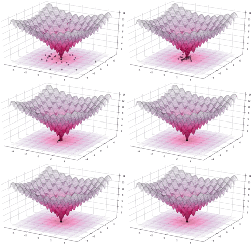
Differential evolution

Differential evolution (DE) is an evolutionary algorithm to optimize a problem by iteratively trying to improve a candidate solution with regard to a given measure of quality. Such methods are commonly known as metaheuristics as they make few or no assumptions about the optimized problem and can search very large spaces of candidate solutions. However, metaheuristics such as DE do not guarantee an optimal solution is ever found.
DE is used for multidimensional real-valued functions but does not use the gradient of the problem being optimized, which means DE does not require the optimization problem to be differentiable, as is required by classic optimization methods such as gradient descent and quasi-newton methods. DE can therefore also be used on optimization problems that are not even continuous, are noisy, change over time, etc.[1]
DE optimizes a problem by maintaining a population of candidate solutions and creating new candidate solutions by combining existing ones according to its simple formulae, and then keeping whichever candidate solution has the best score or fitness on the optimization problem at hand. In this way, the optimization problem is treated as a black box that merely provides a measure of quality given a candidate solution and the gradient is therefore not needed.
History
Storn and Price introduced Differential Evolution in 1995.[2][3][4] Books have been published on theoretical and practical aspects of using DE in parallel computing, multiobjective optimization, constrained optimization, and the books also contain surveys of application areas.[5][6][7][8] Surveys on the multi-faceted research aspects of DE can be found in journal articles.[9][10]
Algorithm
A basic variant of the DE algorithm works by having a population of candidate solutions (called agents). These agents are moved around in the search-space by using simple mathematical formulae to combine the positions of existing agents from the population. If the new position of an agent is an improvement then it is accepted and forms part of the population, otherwise the new position is simply discarded. The process is repeated and by doing so it is hoped, but not guaranteed, that a satisfactory solution will eventually be discovered.
Formally, let be the fitness function which must be minimized (note that maximization can be performed by considering the function instead). The function takes a candidate solution as argument in the form of a vector of real numbers. It produces a real number as output which indicates the fitness of the given candidate solution. The gradient of is not known. The goal is to find a solution for which for all in the search-space, which means that is the global minimum.
Let designate a candidate solution (agent) in the population. The basic DE algorithm can then be described as follows:
- Choose the parameters , , and .
- NP : is the population size, i.e. the number of candidate agents or "parents".
- CR : The parameter is called the crossover probability.
- F : The parameter is called the differential weight.
- Typical settings are , and .
- Optimization performance may be greatly impacted by these choices; see below.
- Initialize all agents with random positions in the search-space.
- Until a termination criterion is met (e.g. number of iterations performed, or adequate fitness reached), repeat the following:
- For each agent in the population do:
- Pick three agents , and from the population at random, they must be distinct from each other as well as from agent . ( is called the "base" vector.)
- Pick a random index where is the dimensionality of the problem being optimized.
- Compute the agent's potentially new position as follows:
- For each , pick a uniformly distributed random number
- If or then set otherwise set . (Index position is replaced for certain.)
- If then replace the agent in the population with the improved or equal candidate solution .
- For each agent in the population do:
- Pick the agent from the population that has the best fitness and return it as the best found candidate solution.
Parameter selection

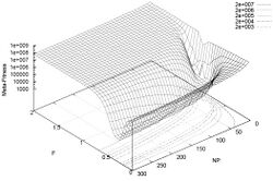
The choice of DE parameters , and can have a large impact on optimization performance. Selecting the DE parameters that yield good performance has therefore been the subject of much research. Rules of thumb for parameter selection were devised by Storn et al.[4][5] and Liu and Lampinen.[11] Mathematical convergence analysis regarding parameter selection was done by Zaharie.[12]
Constraint handling
Differential evolution can be utilized for constrained optimization as well. A common method involves modifying the target function to include a penalty for any violation of constraints, expressed as: . Here, represents either a constraint violation (an L1 penalty) or the square of a constraint violation (an L2 penalty).
This method, however, has certain drawbacks. One significant challenge is the appropriate selection of the penalty coefficient . If is set too low, it may not effectively enforce constraints. Conversely, if it's too high, it can greatly slow down or even halt the convergence process. Despite these challenges, this approach remains widely used due to its simplicity and because it doesn't require altering the differential evolution algorithm itself.
There are alternative strategies, such as projecting onto a feasible set or reducing dimensionality, which can be used for box-constrained or linearly constrained cases. However, in the context of general nonlinear constraints, the most reliable methods typically involve penalty functions.
Variants
Variants of the DE algorithm are continually being developed in an effort to improve optimization performance.[13] The following directions of development can be outlined:
- New schemes for performing crossover and mutation of agents[4]
- Various strategies for handling constraints
- Adaptive strategies that dynamically adjust population size, F and CR parameters
- Specialized algorithms for large-scale optimization
- Multi-objective and many-objective algorithms
- Techniques for handling binary/integer variables
See also
References
- ↑ Rocca, P.; Oliveri, G.; Massa, A. (2011). "Differential Evolution as Applied to Electromagnetics". IEEE Antennas and Propagation Magazine 53 (1): 38–49. doi:10.1109/MAP.2011.5773566. Bibcode: 2011IAPM...53...38R.
- ↑ Storn, Rainer; Price, Kenneth (1995). "Differential evolution—a simple and efficient scheme for global optimization over continuous spaces". International Computer Science Institute (Berkeley) TR (95): TR-95-012. https://cse.engineering.nyu.edu/~mleung/CS909/s04/Storn95-012.pdf. Retrieved 3 April 2024.
- ↑ Storn, R.; Price, K. (1997). "Differential evolution - a simple and efficient heuristic for global optimization over continuous spaces". Journal of Global Optimization 11 (4): 341–359. doi:10.1023/A:1008202821328. Bibcode: 1997JGOpt..11..341S.
- ↑ 4.0 4.1 4.2 Storn, R. (1996). "On the usage of differential evolution for function optimization". pp. 519–523. doi:10.1109/NAFIPS.1996.534789.
- ↑ 5.0 5.1 Price, K.; Storn, R.M.; Lampinen, J.A. (2005). Differential Evolution: A Practical Approach to Global Optimization. Springer. ISBN 978-3-540-20950-8. https://www.springer.com/computer/theoretical+computer+science/foundations+of+computations/book/978-3-540-20950-8.
- ↑ Feoktistov, V. (2006). Differential Evolution: In Search of Solutions. Springer. ISBN 978-0-387-36895-5. https://www.springer.com/mathematics/book/978-0-387-36895-5.
- ↑ Onwubolu, G. C.; Babu, B. V. (2004). New Optimization Techniques in Engineering. Studies in Fuzziness and Soft Computing. 141. doi:10.1007/978-3-540-39930-8. ISBN 978-3-642-05767-0.
- ↑ Chakraborty, U.K., ed. (2008), Advances in Differential Evolution, Springer, ISBN 978-3-540-68827-3, https://www.springer.com/engineering/book/978-3-540-68827-3
- ↑ S. Das; P. N. Suganthan (Feb 2011). "Differential Evolution: A Survey of the State-of-the-art". IEEE Transactions on Evolutionary Computation 15 (1): 4–31. doi:10.1109/TEVC.2010.2059031. https://www.researchgate.net/publication/220380793.
- ↑ S. Das; S. S. Mullick; P. N. Suganthan (2016). "Recent Advances in Differential Evolution - An Updated Survey". Swarm and Evolutionary Computation 27: 1–30. doi:10.1016/j.swevo.2016.01.004. http://web.mysites.ntu.edu.sg/epnsugan/PublicSite/Shared%20Documents/PDFs/DE-Survey-2016.pdf.
- ↑ Liu, J.; Lampinen, J. (2002). "On setting the control parameter of the differential evolution method". Brno, Czech Republic. pp. 11–18.
- ↑ Zaharie, D. (2002). "Critical values for the control parameters of differential evolution algorithms". Brno, Czech Republic. pp. 62–67.
- ↑ Swagatam Das; Sankha Subhra Mullick; P.N. Suganthan (2016). Recent advances in differential evolution.
 |
