Exponential-logarithmic distribution

Short description: Family of lifetime distributions with decreasing failure rate

Exponential-Logarithmic distribution (EL)

Probability density function
Parameters	[math]\displaystyle{ p\in (0,1) }[/math] [math]\displaystyle{ \beta \gt 0 }[/math]
Support	[math]\displaystyle{ x\in[0,\infty) }[/math]
PDF	[math]\displaystyle{ \frac{1}{-\ln p} \times \frac{\beta(1-p) e^{-\beta x}}{1-(1-p) e^{-\beta x}} }[/math]
CDF	[math]\displaystyle{ 1-\frac{\ln(1-(1-p) e^{-\beta x})}{\ln p} }[/math]
Mean	[math]\displaystyle{ -\frac{\text{polylog}(2,1-p)}{\beta\ln p} }[/math]
Median	[math]\displaystyle{ \frac{\ln(1+\sqrt{p})}{\beta} }[/math]
Mode	0
Variance	[math]\displaystyle{ -\frac{2 \text{polylog}(3,1-p)}{\beta^2\ln p} }[/math] [math]\displaystyle{ -\frac{ \text{polylog}^2(2,1-p)}{\beta^2\ln^2 p} }[/math]
MGF	[math]\displaystyle{ -\frac{\beta(1-p)}{\ln p (\beta-t)} \text{hypergeom}_{2,1} }[/math] [math]\displaystyle{ ([1,\frac{\beta-t}{\beta}],[\frac{2\beta-t}{\beta}],1-p) }[/math]

In probability theory and statistics, the Exponential-Logarithmic (EL) distribution is a family of lifetime distributions with decreasing failure rate, defined on the interval [0, ∞). This distribution is parameterized by two parameters [math]\displaystyle{ p\in(0,1) }[/math] and [math]\displaystyle{ \beta \gt 0 }[/math].

Introduction

The study of lengths of the lives of organisms, devices, materials, etc., is of major importance in the biological and engineering sciences. In general, the lifetime of a device is expected to exhibit decreasing failure rate (DFR) when its behavior over time is characterized by 'work-hardening' (in engineering terms) or 'immunity' (in biological terms).

The exponential-logarithmic model, together with its various properties, are studied by Tahmasbi and Rezaei (2008). This model is obtained under the concept of population heterogeneity (through the process of compounding).

Properties of the distribution

Distribution

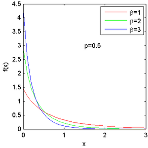
The probability density function (pdf) of the EL distribution is given by Tahmasbi and Rezaei (2008)

[math]\displaystyle{ f(x; p, \beta) := \left( \frac{1}{-\ln p}\right) \frac{\beta(1-p)e^{-\beta x}}{1-(1-p)e^{-\beta x}} }[/math]

where [math]\displaystyle{ p\in (0,1) }[/math] and [math]\displaystyle{ \beta \gt 0 }[/math]. This function is strictly decreasing in [math]\displaystyle{ x }[/math] and tends to zero as [math]\displaystyle{ x\rightarrow \infty }[/math]. The EL distribution has its modal value of the density at x=0, given by

[math]\displaystyle{ \frac{\beta (1-p)}{-p \ln p} }[/math]

The EL reduces to the exponential distribution with rate parameter [math]\displaystyle{ \beta }[/math], as [math]\displaystyle{ p\rightarrow 1 }[/math].

The cumulative distribution function is given by

[math]\displaystyle{ F(x;p,\beta)=1-\frac{\ln(1-(1-p) e^{-\beta x})}{\ln p}, }[/math]

and hence, the median is given by

[math]\displaystyle{ x_\text{median}=\frac{\ln(1+\sqrt{p})}{\beta} }[/math].

Moments

The moment generating function of [math]\displaystyle{ X }[/math] can be determined from the pdf by direct integration and is given by

[math]\displaystyle{ M_X(t) = E(e^{tX}) = -\frac{\beta(1-p)}{\ln p (\beta-t)} F_{2,1}\left(\left[1,\frac{\beta-t}{\beta}\right],\left[\frac{2\beta-t}{\beta}\right],1-p\right), }[/math]

where [math]\displaystyle{ F_{2,1} }[/math] is a hypergeometric function. This function is also known as Barnes's extended hypergeometric function. The definition of [math]\displaystyle{ F_{N,D}({n,d},z) }[/math] is

[math]\displaystyle{ F_{N,D}(n,d,z):=\sum_{k=0}^\infty \frac{ z^k \prod_{i=1}^p\Gamma(n_i+k)\Gamma^{-1}(n_i)}{\Gamma(k+1)\prod_{i=1}^q\Gamma(d_i+k)\Gamma^{-1}(d_i)} }[/math]

where [math]\displaystyle{ n=[n_1, n_2,\dots , n_N] }[/math] and [math]\displaystyle{ {d}=[d_1, d_2, \dots , d_D] }[/math].

The moments of [math]\displaystyle{ X }[/math] can be derived from [math]\displaystyle{ M_X(t) }[/math]. For [math]\displaystyle{ r\in\mathbb{N} }[/math], the raw moments are given by

[math]\displaystyle{ E(X^r;p,\beta)=-r!\frac{\operatorname{Li}_{r+1}(1-p) }{\beta^r\ln p}, }[/math]

where [math]\displaystyle{ \operatorname{Li}_a(z) }[/math] is the polylogarithm function which is defined as follows:

[math]\displaystyle{ \operatorname{Li}_a(z) =\sum_{k=1}^{\infty}\frac{z^k}{k^a}. }[/math]

Hence the mean and variance of the EL distribution are given, respectively, by

[math]\displaystyle{ E(X)=-\frac{\operatorname{Li}_2(1-p)}{\beta\ln p}, }[/math]

[math]\displaystyle{ \operatorname{Var}(X)=-\frac{2 \operatorname{Li}_3(1-p)}{\beta^2\ln p}-\left(\frac{ \operatorname{Li}_2(1-p)}{\beta\ln p}\right)^2. }[/math]

The survival, hazard and mean residual life functions

Hazard function

The survival function (also known as the reliability function) and hazard function (also known as the failure rate function) of the EL distribution are given, respectively, by

[math]\displaystyle{ s(x)=\frac{\ln(1-(1-p)e^{-\beta x})}{\ln p}, }[/math]

[math]\displaystyle{ h(x)=\frac{-\beta(1-p)e^{-\beta x}}{(1-(1-p)e^{-\beta x})\ln(1-(1-p)e^{-\beta x})}. }[/math]

The mean residual lifetime of the EL distribution is given by

[math]\displaystyle{ m(x_0;p,\beta)=E(X-x_0|X\geq x_0;\beta,p)=-\frac{\operatorname{Li}_2(1-(1-p)e^{-\beta x_0})}{\beta \ln(1-(1-p)e^{-\beta x_0})} }[/math]

where [math]\displaystyle{ \operatorname{Li}_2 }[/math] is the dilogarithm function

Random number generation

Let U be a random variate from the standard uniform distribution. Then the following transformation of U has the EL distribution with parameters p and β:

[math]\displaystyle{ X = \frac{1}{\beta}\ln \left(\frac{1-p}{1-p^U}\right). }[/math]

Estimation of the parameters

To estimate the parameters, the EM algorithm is used. This method is discussed by Tahmasbi and Rezaei (2008). The EM iteration is given by

[math]\displaystyle{ \beta^{(h+1)} = n \left( \sum_{i=1}^n\frac{x_i}{1-(1-p^{(h)})e^{-\beta^{(h)}x_i}} \right)^{-1}, }[/math]

[math]\displaystyle{ p^{(h+1)}=\frac{-n(1-p^{(h+1)})} { \ln( p^{(h+1)}) \sum_{i=1}^n \{1-(1-p^{(h)})e^{-\beta^{(h)} x_i}\}^{-1}}. }[/math]

Related distributions

The EL distribution has been generalized to form the Weibull-logarithmic distribution.

If X is defined to be the random variable which is the minimum of N independent realisations from an exponential distribution with rate parameter β, and if N is a realisation from a logarithmic distribution (where the parameter p in the usual parameterisation is replaced by (1 − p)), then X has the exponential-logarithmic distribution in the parameterisation used above.

References

- ↑ 1.0 1.1 1.2 Tahmasbi, R., Rezaei, S., (2008), "A two-parameter lifetime distribution with decreasing failure rate", Computational Statistics and Data Analysis, 52 (8), 3889-3901. doi:10.1016/j.csda.2007.12.002
- ↑ Lewin, L. (1981) Polylogarithms and Associated Functions, North Holland, Amsterdam.
- ↑ Ciumara, Roxana; Preda, Vasile (2009) "The Weibull-logarithmic distribution in lifetime analysis and its properties"[yes|permanent dead link|dead link}}]. In: L. Sakalauskas, C. Skiadas and E. K. Zavadskas (Eds.) Applied Stochastic Models and Data Analysis , The XIII International Conference, Selected papers. Vilnius, 2009 ISBN 978-9955-28-463-5