Failure rate
Failure rate is the frequency with which any system or component fails, expressed in failures per unit of time. It thus depends on the system conditions, time interval, and total number of systems under study.[1] It can describe electronic, mechanical, or biological systems, in fields such as systems and reliability engineering, medicine and biology, or insurance and finance. It is usually denoted by the Greek letter (lambda).
In real-world applications, the failure probability of a system usually differs over time; failures occur more frequently in early-life ("burning in"), or as a system ages ("wearing out"). This is known as the bathtub curve, where the middle region is called the "useful life period".
Mean time between failures (MTBF)
The mean time between failures (MTBF, ) is often reported instead of the failure rate, as numbers such as "2,000 hours" are more intuitive than numbers such as "0.0005 per hour".
However, this is only valid if the failure rate is actually constant over time, such as within the flat region of the bathtub curve. In many cases where MTBF is quoted, it refers only to this region; thus it cannot be used to give an accurate calculation of the average lifetime of a system, as it ignores the "burn-in" and "wear-out" regions.
MTBF appears frequently in engineering design requirements, and governs the frequency of required system maintenance and inspections. A similar ratio used in the transport industries, especially in railways and trucking, is "mean distance between failures" (MDBF) - allowing maintenance to be scheduled based on distance travelled, rather than at regular time intervals.
Mathematical definition
The simplest definition of failure rate is simply the number of failures per time interval :
which would depend on the number of systems under study, and the conditions over the time period.
Failures over time

To accurately model failures over time, a cumulative failure distribution, must be defined, which can be any cumulative distribution function (CDF) that gradually increases from to . In the case of many identical systems, this may be thought of as the fraction of systems failing over time , after all starting operation at time ; or in the case of a single system, as the probability of the system having its failure time before time :
As CDFs are defined by integrating a probability density function, the failure probability density is defined such that:

where is a dummy integration variable. Here can be thought of as the instantaneous failure rate, i.e. the probability of failure in the time interval between and , as tends towards :
Hazard rate
A concept closely related but different[2] to instantaneous failure rate is the hazard rate (or hazard function), . In the many-system case, this is defined as the proportional failure rate of the systems still functioning at time – as opposed to , which is the expressed as a proportion of the initial number of systems.
For convenience we first define the reliability (or survival function) as:
then the hazard rate is simply the instantaneous failure rate, scaled by the fraction of surviving systems at time :
In the probabilistic sense for a single system, this can be interpreted as the instantaneous failure rate under the conditional probability that the system or component has already survived to time :
Conversion to cumulative failure rate
To convert between and , we can solve the differential equation
with initial condition , which yields[2]
Thus for a collection of identical systems, only one of hazard rate , failure probability density , or cumulative failure distribution need be defined.
Confusion can occur as the notation for "failure rate" often refers to the function rather than [3]
Constant hazard rate model
There are many possible functions that could be chosen to represent failure probability density or hazard rate , based on empirical or theoretical evidence, but the most common and easily-understandable choice is to set
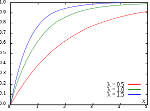
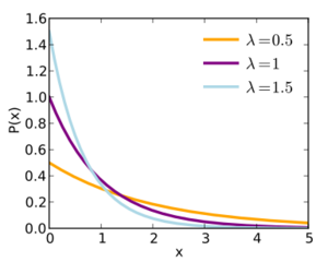
an exponential function with scaling constant . As seen in the figures above, this represents a gradually decreasing failure probability density.
The CDF is then calculated as:
which can be seen to gradually approach as representing the fact that eventually all systems under study will fail.
The hazard rate function is then:
In other words, in this particular case only, the hazard rate is constant over time.
This illustrates the difference in hazard rate and failure probability density - as the number of systems surviving at time gradually reduces, the total failure rate also reduces, but the hazard rate remains constant. In other words, the probabilities of each individual system failing do not change over time as the systems age - they are "memory-less".
Other models

For many systems, a constant hazard function may not be a realistic approximation; the chance of failure of an individual component may depend on its age. Therefore, other distributions are often used.
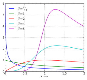
For example, the deterministic distribution increases hazard rate over time (for systems where wear-out is the most important factor), while the Pareto distribution decreases it (for systems where early-life failures are more common). The commonly used Weibull distribution combines both of these effects, as do the log-normal and hypertabastic distributions.
After modelling a given distribution and parameters for , the failure probability density and cumulative failure distribution can be predicted using the given equations.
Measuring failure rate
Failure rate data can be obtained in several ways. The most common means are:
- Estimation
- From field failure rate reports, statistical analysis techniques can be used to estimate failure rates. For accurate failure rates the analyst must have a good understanding of equipment operation, procedures for data collection, the key environmental variables impacting failure rates, how the equipment is used at the system level, and how the failure data will be used by system designers.
- Historical data about the device or system under consideration
- Many organizations maintain internal databases of failure information on the devices or systems that they produce, which can be used to calculate failure rates for those devices or systems. For new devices or systems, the historical data for similar devices or systems can serve as a useful estimate.
- Government and commercial failure rate data
- Handbooks of failure rate data for various components are available from government and commercial sources. MIL-HDBK-217F, Reliability Prediction of Electronic Equipment, is a military standard that provides failure rate data for many military electronic components. Several failure rate data sources are available commercially that focus on commercial components, including some non-electronic components.
- Prediction
- Time lag is one of the serious drawbacks of all failure rate estimations. Often by the time the failure rate data are available, the devices under study have become obsolete. Due to this drawback, failure-rate prediction methods have been developed. These methods may be used on newly designed devices to predict the device's failure rates and failure modes. Two approaches have become well known, Cycle Testing and FMEDA.
- Life Testing
- The most accurate source of data is to test samples of the actual devices or systems in order to generate failure data. This is often prohibitively expensive or impractical, so that the previous data sources are often used instead.
- Cycle Testing
- Mechanical movement is the predominant failure mechanism causing mechanical and electromechanical devices to wear out. For many devices, the wear-out failure point is measured by the number of cycles performed before the device fails, and can be discovered by cycle testing. In cycle testing, a device is cycled as rapidly as practical until it fails. When a collection of these devices are tested, the test will run until 10% of the units fail dangerously.
- FMEDA
- Failure modes, effects, and diagnostic analysis (FMEDA) is a systematic analysis technique to obtain subsystem / product level failure rates, failure modes and design strength. The FMEDA technique considers:
- All components of a design,
- The functionality of each component,
- The failure modes of each component,
- The effect of each component failure mode on the product functionality,
- The ability of any automatic diagnostics to detect the failure,
- The design strength (de-rating, safety factors) and
- The operational profile (environmental stress factors).
Given a component database calibrated with field failure data that is reasonably accurate,[4] the method can predict product level failure rate and failure mode data for a given application. The predictions have been shown to be more accurate[5] than field warranty return analysis or even typical field failure analysis given that these methods depend on reports that typically do not have sufficient detail information in failure records.[6]
Examples
Decreasing failure rates
A decreasing failure rate describes cases where early-life failures are common[7] and corresponds to the situation where is a decreasing function.
This can describe, for example, the period of infant mortality in humans, or the early failure of transistors due to manufacturing defects.
Decreasing failure rates have been found in the lifetimes of spacecraft - Baker and Baker commenting that "those spacecraft that last, last on and on."[8][9]
The hazard rate of aircraft air conditioning systems was found to have an exponentially decreasing distribution.[10]
Renewal processes
In special processes called renewal processes, where the time to recover from failure can be neglected, the likelihood of failure remains constant with respect to time.
For a renewal process with DFR renewal function, inter-renewal times are concave.[clarification needed][11][12] Brown conjectured the converse, that DFR is also necessary for the inter-renewal times to be concave,[13] however it has been shown that this conjecture holds neither in the discrete case[12] nor in the continuous case.[14]
Coefficient of variation
When the failure rate is decreasing the coefficient of variation is ⩾ 1, and when the failure rate is increasing the coefficient of variation is ⩽ 1.[clarification needed][15] Note that this result only holds when the failure rate is defined for all t ⩾ 0[16] and that the converse result (coefficient of variation determining nature of failure rate) does not hold.
Units
Failure rates can be expressed using any measure of time, but hours is the most common unit in practice. Other units, such as miles, revolutions, etc., can also be used in place of "time" units.
Failure rates are often expressed in engineering notation as failures per million, or 10−6, especially for individual components, since their failure rates are often very low.
The Failures In Time (FIT) rate of a device is the number of failures that can be expected in one billion (109) device-hours of operation[17] (e.g. 1,000 devices for 1,000,000 hours, or 1,000,000 devices for 1,000 hours each, or some other combination). This term is used particularly by the semiconductor industry.
Combinations of failure types
If a complex system consists of many parts, and the failure of any single part means the failure of the entire system, and the chance of failure for each part is conditionally independent of the failure of any other part, then the total failure rate is simply the sum of the individual failure rates of its parts
however, this assumes that the failure rate is constant, and that the units are consistent (e.g. failures per million hours), and not expressed as a ratio or as probability densities. This is useful to estimate the failure rate of a system when individual components or subsystems have already been tested.[18][19]
When adding "redundant" components to eliminate a single point of failure, the quantity of interest is not the sum of individual failure rates but rather the "mission failure" rate, or the "mean time between critical failures" (MTBCF).[20]
Combining failure or hazard rates that are time-dependent is more complicated. For example, mixtures of Decreasing Failure Rate (DFR) variables are also DFR.[11] Mixtures of exponentially distributed failure rates are hyperexponentially distributed.
Simple example
Suppose it is desired to estimate the failure rate of a certain component. Ten identical components are each tested until they either fail or reach 1,000 hours, at which time the test is terminated. A total of 7,502 component-hours of testing is performed, and 6 failures are recorded.
The estimated failure rate is:
which could also be expressed as a MTBF of 1,250 hours, or approximately 800 failures for every million hours of operation.
See also
References
- ↑ * MacDiarmid, Preston et al. (n.d.). Reliability Toolkit (Commercial Practices ed.). Rome, New York: Reliability Analysis Center and Rome Laboratory. pp. 35–39.
- ↑ 2.0 2.1 Todinov, MT (2007). "Chapter 2.2 HAZARD RATE AND TIME TO FAILURE DISTRIBUTION". Risk-Based Reliability Analysis and Generic Principles for Risk Reduction.
- ↑ Wang, Shaoping (2016). "Chapter 3.3.1.3: Failure Rate λ(t)". Comprehensive Reliability Design of Aircraft Hydraulic System.
- ↑ Electrical & Mechanical Component Reliability Handbook. exida. 2006. http://www.exida.com.
- ↑ Goble, William M.; Iwan van Beurden (2014). Combining field failure data with new instrument design margins to predict failure rates for SIS Verification. Proceedings of the 2014 International Symposium - BEYOND REGULATORY COMPLIANCE, MAKING SAFETY SECOND NATURE, Hilton College Station-Conference Center, College Station, Texas.
- ↑ W. M. Goble, "Field Failure Data – the Good, the Bad and the Ugly," exida, Sellersville, PA [1]
- ↑ Finkelstein, Maxim (2008). "Introduction". Failure Rate Modelling for Reliability and Risk. Springer Series in Reliability Engineering. pp. 1–84. doi:10.1007/978-1-84800-986-8_1. ISBN 978-1-84800-985-1.
- ↑ Baker, J. C.; Baker, G. A. S. . (1980). "Impact of the space environment on spacecraft lifetimes". Journal of Spacecraft and Rockets 17 (5): 479. doi:10.2514/3.28040. Bibcode: 1980JSpRo..17..479B.
- ↑ Saleh, Joseph Homer; Castet, Jean-François (2011). "On Time, Reliability, and Spacecraft". Spacecraft Reliability and Multi-State Failures. pp. 1. doi:10.1002/9781119994077.ch1. ISBN 9781119994077.
- ↑ Proschan, F. (1963). "Theoretical Explanation of Observed Decreasing Failure Rate". Technometrics 5 (3): 375–383. doi:10.1080/00401706.1963.10490105.
- ↑ 11.0 11.1 Brown, M. (1980). "Bounds, Inequalities, and Monotonicity Properties for Some Specialized Renewal Processes". The Annals of Probability 8 (2): 227–240. doi:10.1214/aop/1176994773.
- ↑ 12.0 12.1 Shanthikumar, J. G. (1988). "DFR Property of First-Passage Times and its Preservation Under Geometric Compounding". The Annals of Probability 16 (1): 397–406. doi:10.1214/aop/1176991910.
- ↑ Brown, M. (1981). "Further Monotonicity Properties for Specialized Renewal Processes". The Annals of Probability 9 (5): 891–895. doi:10.1214/aop/1176994317.
- ↑ Yu, Y. (2011). "Concave renewal functions do not imply DFR interrenewal times". Journal of Applied Probability 48 (2): 583–588. doi:10.1239/jap/1308662647.
- ↑ Wierman, A.; Bansal, N.; Harchol-Balter, M. (2004). "A note on comparing response times in the M/GI/1/FB and M/GI/1/PS queues". Operations Research Letters 32: 73–76. doi:10.1016/S0167-6377(03)00061-0. http://users.cms.caltech.edu/~adamw/papers/fbnote.pdf.
- ↑ Gautam, Natarajan (2012). Analysis of Queues: Methods and Applications. CRC Press. p. 703. ISBN 978-1439806586.
- ↑ Xin Li; Michael C. Huang; Kai Shen; Lingkun Chu. "A Realistic Evaluation of Memory Hardware Errors and Software System Susceptibility". 2010. p. 6.
- ↑ "Reliability Basics". 2010.
- ↑ Vita Faraci. "Calculating Failure Rates of Series/Parallel Networks" . 2006.
- ↑ "Mission Reliability and Logistics Reliability: A Design Paradox".
Further reading
- Goble, William M. (2018), Safety Instrumented System Design: Techniques and Design Verification, Research Triangle Park, NC: International Society of Automation
- Blanchard, Benjamin S. (1992). Logistics Engineering and Management (Fourth ed.). Englewood Cliffs, New Jersey: Prentice-Hall. pp. 26–32. ISBN 0135241170.
- Ebeling, Charles E. (1997). An Introduction to Reliability and Maintainability Engineering. Boston: McGraw-Hill. pp. 23–32. ISBN 0070188521.
- Federal Standard 1037C
- Kapur, K. C.; Lamberson, L. R. (1977). Reliability in Engineering Design. New York: John Wiley & Sons. pp. 8–30. ISBN 0471511919.
- Knowles, D. I. (1995). "Should We Move Away From 'Acceptable Failure Rate'?". Communications in Reliability Maintainability and Supportability (International RMS Committee, USA) 2 (1): 23.
- Modarres, M.; Kaminskiy, M.; Krivtsov, V. (2010). Reliability Engineering and Risk Analysis: A Practical Guide (2nd ed.). CRC Press. ISBN 9780849392474.
- Mondro, Mitchell J. (June 2002). "Approximation of Mean Time Between Failure When a System has Periodic Maintenance". IEEE Transactions on Reliability 51 (2): 166–167. doi:10.1109/TR.2002.1011521. http://www.mitre.org/work/best_papers/02/mondro_approx/mondro_approx.pdf. Retrieved 2008-07-14.
- Rausand, M.; Hoyland, A. (2004). System Reliability Theory; Models, Statistical methods, and Applications. New York: John Wiley & Sons. ISBN 047147133X.
- Turner, T.; Hockley, C.; Burdaky, R. (1997). The Customer Needs A Maintenance-Free Operating Period. Leatherhead, Surrey, UK: ERA Technology Ltd..
- U.S. Department of Defense, (1991) Military Handbook, “Reliability Prediction of Electronic Equipment, MIL-HDBK-217F, 2
External links
- Fault Tolerant Computing in Industrial Automation by Hubert Kirrmann, ABB Research Center, Switzerland
 |
