Fréchet distribution

Short description: Continuous probability distribution

Fréchet

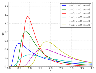
Probability density function
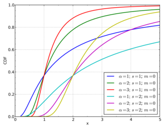
Cumulative distribution function
Parameters	[math]\displaystyle{ \alpha \in (0,\infty) }[/math] shape. (Optionally, two more parameters) [math]\displaystyle{ s \in (0,\infty) }[/math] scale (default: [math]\displaystyle{ s=1 \, }[/math]) [math]\displaystyle{ m \in (-\infty,\infty) }[/math] location of minimum (default: [math]\displaystyle{ m=0 \, }[/math])
Support	[math]\displaystyle{ x\gt m }[/math]
PDF	[math]\displaystyle{ \frac{\alpha}{s} \; \left(\frac{x-m}{s}\right)^{-1-\alpha} \; e^{-(\frac{x-m}{s})^{-\alpha}} }[/math]
CDF	[math]\displaystyle{ e^{-(\frac{x-m}{s})^{-\alpha}} }[/math]
Mean	[math]\displaystyle{ \begin{cases} \ m+s\Gamma\left(1-\frac{1}{\alpha}\right) & \text{for } \alpha\gt 1 \\ \ \infty & \text{otherwise} \end{cases} }[/math]
Median	[math]\displaystyle{ m+\frac{s}{\sqrt[\alpha]{\log_e(2)}} }[/math]
Mode	[math]\displaystyle{ m+s\left(\frac{\alpha}{1+\alpha}\right)^{1/\alpha} }[/math]
Variance	[math]\displaystyle{ \begin{cases} \ s^2\left(\Gamma\left(1-\frac{2}{\alpha}\right)- \left(\Gamma\left(1-\frac{1}{\alpha}\right)\right)^2\right) & \text{for } \alpha\gt 2 \\ \ \infty & \text{otherwise} \end{cases} }[/math]
Skewness	[math]\displaystyle{ \begin{cases} \ \frac{\Gamma\left(1-\frac {3}{\alpha}\right)-3\Gamma\left(1-\frac {2}{\alpha}\right)\Gamma\left(1-\frac {1}{\alpha}\right)+2\Gamma^3\left(1-\frac {1}{\alpha} \right)}{\sqrt{ \left( \Gamma\left(1-\frac{2}{\alpha}\right)-\Gamma^2\left(1-\frac{1}{\alpha}\right) \right)^3 }} & \text{for } \alpha\gt 3 \\ \ \infty & \text{otherwise} \end{cases} }[/math]
Kurtosis	[math]\displaystyle{ \begin{cases} \ -6+ \frac{\Gamma \left(1-\frac{4}{\alpha}\right) -4\Gamma\left(1-\frac{3}{\alpha}\right) \Gamma\left(1-\frac{1}{\alpha}\right)+3 \Gamma^2\left(1-\frac{2}{\alpha} \right)} {\left[\Gamma \left(1-\frac{2}{\alpha}\right) - \Gamma^2 \left(1-\frac{1}{\alpha}\right) \right]^2} & \text{for } \alpha\gt 4 \\ \ \infty & \text{otherwise} \end{cases} }[/math]
Entropy	[math]\displaystyle{ 1 + \frac{\gamma}{\alpha} + \gamma +\ln \left( \frac{s}{\alpha} \right) }[/math], where [math]\displaystyle{ \gamma }[/math] is the Euler–Mascheroni constant.
MGF	Note: Moment [math]\displaystyle{ k }[/math] exists if [math]\displaystyle{ \alpha\gt k }[/math]
CF

The Fréchet distribution, also known as inverse Weibull distribution, is a special case of the generalized extreme value distribution. It has the cumulative distribution function

[math]\displaystyle{ \Pr(X \le x)=e^{-x^{-\alpha}} \text{ if } x\gt 0. }[/math]

where α > 0 is a shape parameter. It can be generalised to include a location parameter m (the minimum) and a scale parameter s > 0 with the cumulative distribution function

[math]\displaystyle{ \Pr(X \le x)=e^{-\left(\frac{x-m}{s}\right)^{-\alpha}} \text{ if } x\gt m. }[/math]

Named for Maurice Fréchet who wrote a related paper in 1927, further work was done by Fisher and Tippett in 1928 and by Gumbel in 1958.

Characteristics

The single parameter Fréchet with parameter [math]\displaystyle{ \alpha }[/math] has standardized moment

[math]\displaystyle{ \mu_k=\int_0^\infty x^k f(x)dx=\int_0^\infty t^{-\frac{k}{\alpha}}e^{-t} \, dt, }[/math]

(with [math]\displaystyle{ t=x^{-\alpha} }[/math]) defined only for [math]\displaystyle{ k\lt \alpha }[/math]:

[math]\displaystyle{ \mu_k=\Gamma\left(1-\frac{k}{\alpha}\right) }[/math]

where [math]\displaystyle{ \Gamma\left(z\right) }[/math] is the Gamma function.

In particular:

• For [math]\displaystyle{ \alpha\gt 1 }[/math] the expectation is [math]\displaystyle{ E[X]=\Gamma(1-\tfrac{1}{\alpha}) }[/math]
• For [math]\displaystyle{ \alpha\gt 2 }[/math] the variance is [math]\displaystyle{ \text{Var}(X)=\Gamma(1-\tfrac{2}{\alpha})-\big(\Gamma(1-\tfrac{1}{\alpha})\big)^2. }[/math]

The quantile [math]\displaystyle{ q_y }[/math] of order [math]\displaystyle{ y }[/math] can be expressed through the inverse of the distribution,

[math]\displaystyle{ q_y=F^{-1}(y)=\left(-\log_e y \right)^{-\frac{1}{\alpha}} }[/math].

In particular the median is:

[math]\displaystyle{ q_{1/2}=(\log_e 2)^{-\frac{1}{\alpha}}. }[/math]

The mode of the distribution is [math]\displaystyle{ \left(\frac{\alpha}{\alpha+1}\right)^\frac{1}{\alpha}. }[/math]

Especially for the 3-parameter Fréchet, the first quartile is [math]\displaystyle{ q_1= m+\frac{s}{\sqrt[\alpha]{\log(4)}} }[/math] and the third quartile [math]\displaystyle{ q_3= m+\frac{s}{\sqrt[\alpha]{\log(\frac{4}{3})}}. }[/math]

Also the quantiles for the mean and mode are:

[math]\displaystyle{ F(mean)=\exp \left( -\Gamma^{-\alpha} \left(1- \frac{1}{\alpha} \right) \right) }[/math]

[math]\displaystyle{ F(mode)=\exp \left( -\frac{\alpha+1}{\alpha} \right). }[/math]

Applications

File:FitFrechetDistr.tif

• In hydrology, the Fréchet distribution is applied to extreme events such as annually maximum one-day rainfalls and river discharges. The blue picture, made with CumFreq, illustrates an example of fitting the Fréchet distribution to ranked annually maximum one-day rainfalls in Oman showing also the 90% confidence belt based on the binomial distribution. The cumulative frequencies of the rainfall data are represented by plotting positions as part of the cumulative frequency analysis.

However, in most hydrological applications, the distribution fitting is via the generalized extreme value distribution as this avoids imposing the assumption that the distribution does not have a lower bound (as required by the Frechet distribution).

Fitted decline curve analysis. Duong model can be thought of as a generalization of the Frechet distribution.

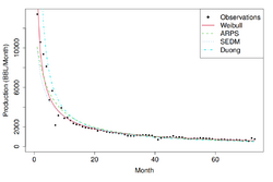
• In decline curve analysis, a declining pattern the time series data of oil or gas production rate over time for a well can be described by the Fréchet distribution.
• One test to assess whether a multivariate distribution is asymptotically dependent or independent consists of transforming the data into standard Fréchet margins using the transformation [math]\displaystyle{ Z_i = -1/\log F_i(X_i) }[/math] and then mapping from Cartesian to pseudo-polar coordinates [math]\displaystyle{ (R, W)= (Z_1 + Z_2, Z_1/(Z_1 + Z_2)) }[/math]. Values of [math]\displaystyle{ R \gg 1 }[/math] correspond to the extreme data for which at least one component is large while [math]\displaystyle{ W }[/math] approximately 1 or 0 corresponds to only one component being extreme.
• In Economics it is used to model the idiosyncratic component of preferences of individuals for different products (Industrial Organization), locations (Urban Economics), or firms (Labor Economics).

Related distributions

• If [math]\displaystyle{ X \sim U(0,1) \, }[/math] (Uniform distribution (continuous)) then [math]\displaystyle{ m + s(-\log(X))^{-1/\alpha} \sim \textrm{Frechet}(\alpha,s,m)\, }[/math]
• If [math]\displaystyle{ X \sim \textrm{Frechet}(\alpha,s,m)\, }[/math] then [math]\displaystyle{ k X + b \sim \textrm{Frechet}(\alpha,k s,k m + b)\, }[/math]
• If [math]\displaystyle{ X_i \sim \textrm{Frechet}(\alpha,s,m) \, }[/math] and [math]\displaystyle{ Y=\max\{\,X_1,\ldots,X_n\,\} \, }[/math] then [math]\displaystyle{ Y \sim \textrm{Frechet}(\alpha,n^{\tfrac{1}{\alpha}} s,m) \, }[/math]
• The cumulative distribution function of the Frechet distribution solves the maximum stability postulate equation
• If [math]\displaystyle{ X \sim \textrm{Frechet}(\alpha,s,m=0)\, }[/math] then its reciprocal is Weibull-distributed: [math]\displaystyle{ X^{-1} \sim \textrm{Weibull}(k=\alpha, \lambda=s^{-1})\, }[/math]

Properties

• The Frechet distribution is a max stable distribution
• The negative of a random variable having a Frechet distribution is a min stable distribution

See also

• Type-2 Gumbel distribution
• Fisher–Tippett–Gnedenko theorem

Further reading

• Kotz, S.; Nadarajah, S. (2000). Extreme Value Distributions: Theory and applications. World Scientific. ISBN 1-86094-224-5. 

External links

• Hurairah, Ahmed; Ibrahim, Noor Akma; bin Daud, Isa; Haron, Kassim (February 2005). "An application of a new extreme value distribution to air pollution data". Management of Environmental Quality 16 (1): 17–25. doi:10.1108/14777830510574317. ISSN 1477-7835. 
• "wfrechstat: Mean and variance for the Frechet distribution". Lund University / Lund Institute of Technology. https://www.maths.lth.se/matstat/wafo/documentation/wafodoc/wafo/wstats/wfrechstat.html.

References

- ↑ 1.0 1.1 Muraleedharan, G.; Guedes Soares, C.; Lucas, Cláudia (2011). Wright, Linda L.. ed. Sea Level Rise, Coastal Engineering, Shorelines, and Tides. Nova Science Publishers. Chapter 14, pp. 269–276. ISBN 978-1-61728-655-1.
- ↑ Khan, M.S.; Pasha, G.R.; Pasha, A.H. (February 2008). "Theoretical analysis of inverse Weibull distribution". WSEAS Transactions on Mathematics 7 (2): 30–38. http://www.wseas.us/e-library/transactions/mathematics/2008/theoretical.pdf.
- ↑ de Gusmão, Felipe R.S.; Ortega, Edwin M.M.; Cordeiro, Gauss M. (2011). "The generalized inverse Weibull distribution". Statistical Papers (Springer-Verlag) 52 (3): 591–619. doi:10.1007/s00362-009-0271-3. ISSN 0932-5026.
- ↑ Fréchet, M. (1927). "Sur la loi de probabilité de l'écart maximum". Annales Polonici Mathematici 6: 93.
- ↑ Fisher, R.A.; Tippett, L.H.C. (1928). "Limiting forms of the frequency distribution of the largest and smallest member of a sample". Proceedings of the Cambridge Philosophical Society 24 (2): 180–190. doi:10.1017/S0305004100015681. Bibcode: 1928PCPS...24..180F.
- ↑ Gumbel, E.J. (1958). Statistics of Extremes. New York, NY: Columbia University Press. OCLC 180577.
- ↑ Coles, Stuart (2001). An Introduction to Statistical Modeling of Extreme Values. Springer-Verlag. ISBN 978-1-85233-459-8. https://books.google.com/books?id=2nugUEaKqFEC&pg=PP1.
- ↑ Lee, Se Yoon; Mallick, Bani (2021). "Bayesian Hierarchical Modeling: Application Towards Production Results in the Eagle Ford Shale of South Texas". Sankhya B 84: 1–43. doi:10.1007/s13571-020-00245-8.