Fundamental polygon

In mathematics, a fundamental polygon can be defined for every compact Riemann surface of genus greater than 0. It encodes not only the topology of the surface through its fundamental group but also determines the Riemann surface up to conformal equivalence. By the uniformization theorem, every compact Riemann surface has simply connected universal covering surface given by exactly one of the following:

• the Riemann sphere,
• the complex plane,
• the unit disk D or equivalently the upper half-plane H.

In the first case of genus zero, the surface is conformally equivalent to the Riemann sphere.

In the second case of genus one, the surface is conformally equivalent to a torus C/Λ for some lattice Λ in C. The fundamental polygon of Λ, if assumed convex, may be taken to be either a period parallelogram or a centrally symmetric hexagon, a result first proved by Fedorov in 1891.

In the last case of genus g > 1, the Riemann surface is conformally equivalent to H/Γ where Γ is a Fuchsian group of Möbius transformations. A fundamental domain for Γ is given by a convex polygon for the hyperbolic metric on H. These can be defined by Dirichlet polygons and have an even number of sides. The structure of the fundamental group Γ can be read off from such a polygon. Using the theory of quasiconformal mappings and the Beltrami equation, it can be shown there is a canonical convex Dirichlet polygon with 4g sides, first defined by Fricke, which corresponds to the standard presentation of Γ as the group with 2g generators a₁, b₁, a₂, b₂, ..., a_g, b_g and the single relation [a₁,b₁][a₂,b₂] ⋅⋅⋅ [a_g,b_g] = 1, where [a,b] = a b a⁻¹b⁻¹.

Any Riemannian metric on an oriented closed 2-manifold M defines a complex structure on M, making M a compact Riemann surface. Through the use of fundamental polygons, it follows that two oriented closed 2-manifolds are classified by their genus, that is half the rank of the Abelian group Γ/[Γ,Γ], where Γ = π₁(M). Moreover, it also follows from the theory of quasiconformal mappings that two compact Riemann surfaces are diffeomorphic if and only if they are homeomorphic. Consequently, two closed oriented 2-manifolds are homeomorphic if and only if they are diffeomorphic. Such a result can also be proved using the methods of differential topology.

Fundamental polygons in genus one

Parallelograms and centrally symmetric hexagons

In the case of genus one, a fundamental convex polygon is sought for the action by translation of Λ = Z a ⊕ Z b on R² = C where a and b are linearly independent over R. (After performing a real linear transformation on R², it can be assumed if necessary that Λ = Z² = Z + Z i; for a genus one Riemann surface it can be taken to have the form Λ = Z² = Z + Z ω, with Im ω > 0.) A fundamental domain is given by the parallelogram s x + t y for 0 < s , t < 1 where x and y are generators of Λ.

If C is the interior of a fundamental convex polygon, then the translates C + x cover R² as x runs over Λ. It follows that the boundary points of C are formed of intersections C ∩ (C + x). These are compact convex sets in ∂C and thus either vertices of C or sides of C. It follows that every closed side of C can be written this way. Translating by −x it follows that C ∩ (C − x) is also a side of C. Thus sides of C occur in parallel pairs of equal length. The end points of two such parallel segments of equal length can be joined so that they intersect and the intersection occurs at the midpoints of the line segments joining the endpoints. It follows that the intersections of al such segments occur at the same point. Translating that point to the origin, it follows that the polygon is centrally symmetric; that is, if a point z is in the polygon, so too is −z.

It is easy to see translates of a centrally symmetric convex hexagon tessellate the plane. If A is a point of the hexagon, then the lattice is generated by the displacement vectors AB and AC where B and C are the two vertices which are not neighbours of A and not opposite A. Indeed, the second picture shows how the hexagon is equivalent to the parallelogram obtained by displacing the two triangles chopped off by the segments AB and AC. Equally well the first picture shows another way of matching a tiling by parallelograms with the hexagonal tiling. If the centre of the hexagon is 0 and the vertices in order are a, b, c, −a, −b and −c, then Λ is the Abelian group with generators a + b and b + c.

Examples of Fundamental Polygons Generated by Parallelograms

There are exactly four topologies that can be created by identifying the sides of a rhombus in different ways. They are given below as directional edges A and B on a square, either as AABB or ABAB sequences.

Name	Sphere	Torus	Projective plane	Klein bottle
Orientable	Yes		No
Total curvature	4π	0	2π	0
Topology ABAB (square)		[math]\displaystyle{ A B A^{-1} B^{-1} }[/math]	[math]\displaystyle{ A B A B }[/math]	[math]\displaystyle{ A B A B^{-1} }[/math] (or [math]\displaystyle{ A B A^{-1} B }[/math])
Topology AABB (square)	[math]\displaystyle{ A B B^{-1} A^{-1} }[/math]		[math]\displaystyle{ A B B^{-1} A }[/math] (or [math]\displaystyle{ A B B A^{-1} }[/math])	[math]\displaystyle{ A B B A }[/math]
Geometry	Sphere	Torus	Hemisphere	Half torus

Fedorov's theorem

Fedorov's theorem, established by the Russian crystallographer Evgraf Fedorov in 1891, asserts that parallelograms and centrally symmetric hexagons are the only convex polygons that are fundamental domains. There are several proofs of this, some of the more recent ones related to results in convexity theory, the geometry of numbers and circle packing, such as the Brunn–Minkowski inequality. Two elementary proofs due to H. S. M. Coxeter and Voronoi will be presented here.

Coxeter's proof proceeds by assuming that there is a centrally symmetric convex polygon C with 2m sides. Then a large closed parallelogram formed from N² fundamental parallelograms is tiled by translations of C which go beyond the edges of the large parallelogram. This induces a tiling on the torus C/NΛ. Let v, e and f be the number of vertices, edges and faces in this tiling (taking into account identifications in the quotient space). Then, because the Euler–Poincaré characteristic of a torus is zero,

[math]\displaystyle{ v - e + f =0. }[/math]

On the other hand, since each vertex is on at least 3 different edges and every edge is between two vertices,

[math]\displaystyle{ 3v\le 2e. }[/math]

Moreover, since every edge is on exactly two faces,

[math]\displaystyle{ 2e = 2mf. }[/math]

Hence

[math]\displaystyle{ mf= e \le 3(e-v)=3f. }[/math]

so that

[math]\displaystyle{ m\le 3, }[/math]

as required.

Voronoi's proof starts with the observation that every edge of C corresponds to an element x of Λ. In fact the edge is the orthogonal bisector of the radius from 0 to x. Hence the foot of the perpendicular from 0 to each edge lies in the interior of each edge. If y is any lattice point, then 1/2 y cannot lie in C; for if so, –1/2 y would also lie in C, contradicting C being a fundamental domain for Λ. Let ±x₁, ..., ±x_m be the 2m distinct points of Λ corresponding to sides of C. Fix generators a and b of Λ. Thus x_i = α_i a + β_i b, where α_i and β_i are integers. It is not possible for both α_i and β_i to be even, since otherwise ± 1/2 x_i would be a point of Λ on a side, which contradicts C being a fundamental domain. So there are three possibilities for the pair of integers (α_i, β_i) modulo 2: (0,1), (1,0) and (1,1). Consequently, if m > 3, there would be x_i and x_j with i ≠ j with both coordinates of x_i − x_j even, i.e. 1/2 (x_i + x_j) lies in Λ. But this is the midpoint of the line segment joining two interior points of edges and hence lies in C, the interior of the polygon. This again contradicts the fact that C is a fundamental domain. So reductio ad absurdum m ≤ 3, as claimed.

Dirichlet–Voronoi domains

For a lattice Λ in C = R², a fundamental domain can be defined canonically using the conformal structure of C. Note that the group of conformal transformations of C is given by complex affine transformations g(z) = az + b with a ≠ 0. These transformations preserve Euclidean metric d(z, w) = |z − w| up to a factor, as well as preserving the orientation. It is the subgroup of the Möbius group fixing the point at ∞. The metric structure can be used to define a canonical fundamental domain by C = {z: d(z, 0) < d(z, λ) for all λ ≠ 0 in Λ}. (It is obvious from the definition that it is a fundamental domain.) This is an example of a Dirichlet domain or Voronoi diagram: since complex translations form an Abelian group, so commute with the action of Λ, these concepts coincide. The canonical fundamental domain for Λ = Z + Zω with Im ω > 0 is either a symmetric convex parallelogram or hexagon with centre 0. By conformal equivalence, the period ω can be further restricted to satisfy |Re ω| ≤ 1/2 and |ω| ≥ 1. As Dirichlet showed ("Dirichlet's hexagon theorem", 1850), for almost all ω the fundamental domain is a hexagon. For Re ω > 0, the midpoints of sides are given by ±1/2, ±ω/2 and ±(ω – 1)/2; the sides bisect the corresponding radii from 0 orthogonally, which determines the vertices completely. In fact the first vertex must have the form (1 + ix)/2 and ω(1 + iy)/2 with x and y real; so if ω = a + ib, then a – by = 1 and x = b + ay. Hence y = (a – 1)/b and x = (a² + b² – a)/b. The six vertices are therefore ±ω(1 – iy)/2 and ±(1 ± ix)/2.

Fundamental polygons in higher genus

Overview

Every compact Riemann surface X has a universal covering surface which is a simply connected Riemann surface X. The fundamental group of X acts as deck transformations of X and can be identified with a subgroup Γ of the group of biholomorphisms of X. The group Γ thus acts freely on X with compact quotient space X/Γ, which can be identified with X. Thus the classification of compact Riemann surfaces can be reduced to the study of possible groups Γ. By the uniformization theorem X is either the Riemann sphere, the complex plane or the unit disk/upper halfplane. The first important invariant of a compact Riemann surface is its genus, a topological invariant given by half the rank of the Abelian group Γ/[Γ, Γ] (which can be identified with the homology group H₁(X, Z)). The genus is zero if the covering space is the Riemann sphere; one if it is the complex plane; and greater than one if it is the unit disk or upper halfplane.

Bihomolomorphisms of the Riemann sphere are just complex Möbius transformations and every non-identity transformation has at least one fixed point, since the corresponding complex matrix always has at least one non-zero eigenvector. Thus if X is the Riemann sphere, then X must be simply connected and biholomorphic to the Riemann sphere, the genus zero Riemann surface. When X is the complex plane, the group of biholomorphisms is the affine group, the complex Möbius transformations fixing ∞, so the transformations g(z) = az + b with a ≠ 0. The non-identity transformations without fixed points are just those with a = 1 and b ≠ 0, i.e. the non-zero translations. The group Γ can thus be identified with a lattice Λ in C and X with a quotient C/Λ, as described in the section on fundamental polygons in genus one. In the third case when X is the unit disk or upper half plane, the group of biholomorphisms consists of the complex Möbius transformations fixing the unit circle or the real axis. In the former case, the transformations correspond to elements of the group SU(1, 1)/{±I}; in the latter case they correspond to real Möbius transformations, so elements of SL(2, R)/{±I}.

The study and classification of possible groups Γ that act freely on the unit disk or upper halfplane with compact quotient—the Fuchsian groups of the first kind—can be accomplished by studying their fundamental polygons, as described below. As Poincaré observed, each such polygon has special properties, namely it is convex and has a natural pairing between its sides. These not only allow the group to be recovered but provide an explicit presentation of the group by generators and relations. Conversely Poincaré proved that any such polygon gives rise to a compact Riemann surface; in fact, Poincaré's polygon theorem applied to more general polygons, where the polygon was allowed to have ideal vertices, but his proof was complete only in the compact case, without such vertices. Without assumptions on the convexity of the polygon, complete proofs have been given by Maskit and de Rham, based on an idea of Siegel, and can be found in (Beardon 1983), (Iversen 1992) and (Stillwell 1992). Carathéodory gave an elementary treatment of the existence of tessellations by Schwarz triangles, i.e. tilings by geodesic triangles with angles π/a, π/b, π/c with sum less than π where a, b, c are integers. When all the angles equal π/2g, this establishes the tiling by regular 4g-sided hyperbolic polygons and hence the existence of a particular compact Riemann surface of genus g as a quotient space. This special example, which has a cyclic group Z_2g of bihomolomorphic symmetries, is used in the development below.

The classification up to homeomorphism and diffeomorphism of compact Riemann surfaces implies the classification of closed orientable 2-manifolds up to homeomorphism and diffeomorphism: any two 2-manifolds with the same genus are diffeomorphic. In fact using a partition of unity, every closed orientable 2-manifold admits a Riemannian metric. For a compact Riemann surface a conformal metric can also be introduced which is conformal, so that in holomorphic coordinates the metric takes the form ρ(z) |dz|². Once this metric has been chosen, locally biholomorphic mappings are precisely orientation-preserving diffeomorphisms that are conformal, i.e. scale the metric by a smooth function. The existence of isothermal coordinates—which can be proved using either local existence theorems for the Laplacian or the Beltrami equation—shows that every closed oriented Riemannian 2-manifold can be given a complex structure compatible with its metric, and hence has the structure of a compact Riemann surface. This construction shows that the classification of closed orientable 2-manifolds up to diffeomorphism or homeomorphism can be reduced to the case of compact Riemann surfaces.

The classification up to homeomorphism and diffeomorphism of compact Riemann surfaces can be accomplished using the fundamental polygon. Indeed, as Poincaré observed, convex fundamental polygons for compact Riemann surfaces H/Γ can be constructed by adapting the method of Dirichlet from the Euclidean space to hyperbolic space. Then following Nevanlinna and Jost, the fundamental domain can be modified in steps to yield a non-convex polygon with vertices lying in a single orbit of Γ and piecewise geodesic sides. The pairing relation on the sides is also modified in each of these steps. Each step involves cutting the polygon by a diagonal geodesic segment in the interior of the polygon and reassembling the polygon using one of the Möbius transformations involved in the pairing. No two paired sides can have a common vertex in the final pairing relation, which satisfies similar properties to the original relation. This polygon can in turn be successively modified by reassembling the polygon after cutting it by a diagonal piecewise geodesic segment in its interior. The final polygon has 4g equivalent vertices, with sides that are piecewise geodesic. The sides are labelled by the group elements which give the Möbius transformation to the paired side. In order the labelling is

[math]\displaystyle{ a_1, b_1, a_1^{-1}, b_1^{-1}, \dots, a_g, b_g, a_g^{-1}, b_g^{-1}, }[/math]

so that Γ is generated by the a_i and b_i subject to the single relation

[math]\displaystyle{ a_1b_1a_1^{-1}b_1^{-1} \cdots a_g b_g a_g^{-1} b_g^{-1} = 1. }[/math]

• 

  Genus zero surface (sphere)

• 

  Genus one surface (torus)

• 

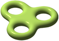
  Genus two surface

• 

  Genus three surface

Using the theory of intersection numbers, it follows that the shape obtained by joining vertices by geodesics is also a proper polygon, not necessarily convex, and is also a fundamental domain with the same group elements giving the pairing. This yields a fundamental polygon with edges given by geodesic segments and with the standard labelling. The abelianisation of Γ, the quotient group Γ/[Γ, Γ], is a free Abelian group with 2g generators. Thus the genus g is a topological invariant. It is easy to see that two Riemann surfaces with the same genus are homeomorphic since as topological space since they are obtained by identifying sides of a 4g-sided polygon—a Euclidean polygon in the Klein model—by diffeomorphisms between paired sides. Applying this construction to the regular 4g-sided polygon allows the Riemann surface to be viewed topologically as a doughnut with g holes, the standard description of oriented surfaces in introductory texts on topology.

There are several further results:

• Two homeomorphic Riemann surfaces are diffeomorphic.
• Any convex fundamental polygon in genus g has N vertices where 4g ≤ N ≤ 12g – 6.
• A Dirichlet polygon in genus g has exactly 12g – 6 vertices for a dense open set of centres.
• Every genus g Riemann surface has a Fricke fundamental polygon, i.e. a convex polygon with canonical pairing between sides. (The polygon need not necessarily be a Dirichlet polygon.)
• After a suitable normalisation and labelling of the generators of the fundamental group, the Fricke polygon is uniquely determined and the 6g – 6 real parameters describing it can be used as global real analytic parameters for Teichmüller space in genus g.

These results are tied up with the interrelation between homeomorphisms and the fundamental group: this reflects the fact that the mapping class group of a Riemann surface—the group of quasiconformal self-homomorphisms of a Riemann surface H/Γ modulo those homotopic to the identity—can be identified with the outer automorphism group of Γ (the Dehn–Nielsen–Baer theorem). To see this connection, note that if f is a quasiconformal homeomorphism of X₁ = H/Γ₁ onto X₂ = H/Γ₂, then f lifts to a quasiconformal homeomorphism f of H onto itself. This lift is unique up to pre-composition with elements of Γ₁ and post-composition with elements of Γ₂. If π_i is the projection of H onto X_i, then f ∘ π₁ = π₂ ∘ f and Γ_i is just the group of homeomorphisms g of H such that π_i ∘ g = π_i. If follows that f g = θ(g) f for g in Γ₁ where θ is a group isomorphism of Γ₁ onto Γ₂. A different choice of f changes θ by composition with an inner automorphism: such isomorphisms are said to be equivalent.

Two isomorphisms θ and θ′ are equivalent if and only if the corresponding homeomorphisms f and f' are homotopic. In fact it suffices to show that a quasiconformal self-homeomorphism f of a surface induces an inner automorphism of the fundamental group if and only if it is homotopic to the identity map: in other words the homomorphism of the quasiconformal self-homeomorphism group of H/Γ into Out Γ passes to the mapping class group on which it is injective. Indeed, suppose first that F(t) is a continuous path of self-homeomorphisms with F(0) = id and F(1) = f. Then there is a continuous lift F(t) with F(0) = id. Moreover, for each g in Γ, F(t) ∘ g ∘ F(t)⁻¹ is a continuously varying element of Γ equal to g for t = 0; so discreteness of Γ forces this element to be constant and hence equal to g so that F(t) commutes with Γ, so F(1) induces the trivial automorphism. If on the other hand F is a quasiconformal lift of f inducing an inner automorphism of Γ, after composition with an element Γ if necessary it can be assumed that F commutes with Γ. Since F is quasiconformal, it extends to a quasisymmetric homeomorphism of the circle which also commutes with Γ. Each g ≠ id in Γ is hyperbolic so has two fixed points on the circle a_± such that for all other points z, g^±n(z) tends to a_± as n tends to infinity. Hence F must fix these points; since these points are dense in the circle as g varies, it follows that F fixes the unit circle. Let μ = F_z / F_z, so that μ is a Γ-invariant Beltrami differential. Let F(t) be the solution of the Beltrami equation tμ normalised to fix three points on the unit circle. Then F(t) commutes with Γ and so, as for F = F(1), is the identity on the unit circle. By construction F(t) is an isotopy between the identity and F. This proves injectivity.

The proof of surjectivity relies on comparing the hyperbolic metric on D with a word-length metric on Γ. Assuming without loss of generality that 0 lies in the interior of a convex fundamental polygon C and g is an element of Γ, the ray from 0 to g(0)—the hyperbolic geodesic—passes through a succession of translates of C. Each of these is obtained from the previous one by applying a generator of Γ or a fixed product of generators (if successive translates meet in a vertex). It follows that the hyperbolic distance between 0 and g(0) is less than 4g times the word length of g plus twice diameter of the fundamental polygon. Thus the metric on Γ d₁(g, h) = L(h⁻¹g) defined by the word length L(g) satisfies

[math]\displaystyle{ d(g(0),h(0)) \le a\, d_1(g,h) + b }[/math]

for positive constants a and b. Conversely there are positive constants c and d such that

[math]\displaystyle{ d_1(g,h) \le c \,d(g(0),h(0)) + d. }[/math]

Dirichlet polygons

Given a point [math]\displaystyle{ z_0 }[/math] in the upper half-plane H, and a discrete subgroup Γ of PSL(2, R) that acts freely discontinuously on the upper half-plane, then one can define the Dirichlet polygon as the set of points

[math]\displaystyle{ F=\{z \in \mathbf{H} : d(z,z_0) \lt d(z,gz_0) \;\; \forall g\in \Gamma, g\ne 1 \} }[/math]

Here, d is a hyperbolic metric on the upper half-plane. The metric fundamental polygon is more usually called the Dirichlet polygon.

• This fundamental polygon is a fundamental domain.
• This fundamental polygon is convex in that the geodesic joining any two points of the polygon is contained entirely inside the polygon.
• The diameter of F is less than or equal to the diameter of H/Γ. In particular, the closure of F is compact.
• If Γ has no fixed points in H and H/Γ is compact, then F will have finitely many sides.
• Each side of the polygon is a geodesic arc.
• For every side s of the polygon, there is precisely one other side s′ such that gs = s′ for some g in Γ. Thus, this polygon will have an even number of sides.
• The set of group elements g that join sides to each other are generators of Γ (note though that this set of generators is not necessarily minimal).
• The upper half-plane is tiled by the closure of F under the action of Γ. That is, [math]\displaystyle{ H=\cup_{g\in\Gamma}\, g\overline{F} }[/math] where [math]\displaystyle{ \overline{F} }[/math] is the closure of F.

Normalised polygon

In this section, starting from an arbitrary Dirichlet polygon, a description will be given of the method of (Nevanlinna 1953), elaborated in (Jost 2002), for modifying the polygon to a non-convex polygon with 4g equivalent vertices and a canonical pairing on the sides. This treatment is an analytic counterpart of the classical topological classification of orientable 2-dimensional polyhedra presented in (Seifert Threlfall).

Fricke canonical polygon

Given a Riemann surface of genus g greater than one, Fricke described another fundamental polygon, the Fricke canonical polygon, which is a very special example of a Dirichlet polygon. The polygon is related to the standard presentation of the fundamental group of the surface. Fricke's original construction is complicated and described in (Fricke Klein). Using the theory of quasiconformal mappings of Ahlfors and Bers, (Keen 1965) gave a new, shorter and more precise version of Fricke's construction. The Fricke canonical polygon has the following properties:

• The vertices of the Fricke polygon has 4g vertices which all lie in an orbit of Γ. By vertex is meant the point where two sides meet.
• The sides are matched in distinct pairs, so that there is a unique element of Γ carrying a side to the paired side, reversing the orientation. Since the action of Γ is orientation-preserving, if one side is called [math]\displaystyle{ A }[/math], then the other of the pair can be marked with the opposite orientation [math]\displaystyle{ A^{-1} }[/math].
• The edges of the standard polygon can be arranged so that the list of adjacent sides takes the form [math]\displaystyle{ A_1 B_1 A_1^{-1} B_1^{-1}A_2 B_2 A_2^{-1} B_2^{-1}\cdots A_g B_g A_g^{-1} B_g^{-1} }[/math]. That is, pairs of sides can be arranged so that they interleave in this way.
• The sides are geodesic arcs.
• Each of the interior angles of the Fricke polygon is strictly less than π, so that the polygon is strictly convex, and the sum of these interior angles is 2π.

The above construction is sufficient to guarantee that each side of the polygon is a closed (non-trivial) loop in the Riemann surface H/Γ. As such, each side can thus an element of the fundamental group [math]\displaystyle{ \pi_1 (\mathbb{H}/\Gamma) \equiv \Gamma }[/math]. In particular, the fundamental group [math]\displaystyle{ \pi_1 (\mathbb{H}/\Gamma) }[/math] has 2g generators [math]\displaystyle{ A_1, B_1, A_2, B_2, \cdots A_g, B_g }[/math], with exactly one defining constraint,

[math]\displaystyle{ A_1 B_1 A_1^{-1} B_1^{-1}A_2 B_2 A_2^{-1} B_2^{-1}\cdots A_g B_g A_g^{-1} B_g^{-1}=1 }[/math].

The genus of the Riemann surface H/Γ is g.

Area

The area of the standard fundamental polygon is [math]\displaystyle{ 4\pi(g-1) }[/math] where g is the genus of the Riemann surface (equivalently, where 4g is the number of the sides of the polygon). Since the standard polygon is a representative of H/Γ, the total area of the Riemann surface is equal to the area of the standard polygon. The area formula follows from the Gauss–Bonnet theorem and is in a certain sense generalized through the Riemann–Hurwitz formula.

Explicit form for standard polygons

Explicit expressions can be given for the regular standard 4g-sided polygon, with rotational symmetry. In this case, that of a genus [math]\displaystyle{ g }[/math] Riemann surface with g-fold rotational symmetry, the group may be given by [math]\displaystyle{ 2g }[/math] generators [math]\displaystyle{ a_k }[/math]. These generators are given by the following fractional linear transforms acting on the upper half-plane:

[math]\displaystyle{ a_k= \left( \begin{matrix} \cos k\alpha & -\sin k\alpha \\ \sin k\alpha & \cos k\alpha \end{matrix} \right) \left( \begin{matrix} e^p & 0 \\ 0 & e^{-p} \end{matrix} \right) \left( \begin{matrix} \cos k\alpha & \sin k\alpha \\ -\sin k\alpha & \cos k\alpha \end{matrix} \right) }[/math]

for [math]\displaystyle{ 0\le k \lt 2g }[/math]. The parameters are given by

[math]\displaystyle{ \alpha= \frac{\pi}{4g}\left(2g-1\right) }[/math]

and

[math]\displaystyle{ \beta= \frac{\pi}{4g} }[/math]

and

[math]\displaystyle{ p=\ln \frac{\cos \beta + \sqrt{\cos 2\beta}}{\sin \beta} }[/math]

It may be verified that these generators obey the constraint

[math]\displaystyle{ a_0a_1\cdots a_{2g-1} a^{-1}_0a^{-1}_1\cdots a^{-1}_{2g-1}=1 }[/math]

which gives the totality of the group presentation.

See also

• Cayley graph
• Euclidean domain
• Voronoi diagram

References

• Ahlfors, Lars V. (2006), Lectures on quasiconformal mappings, University Lecture Series, 38 (Second ed.), American Mathematical Society, ISBN 978-0-8218-3644-6 
• Appell, P.; Goursat, E.; Fatou, P. (1930), Théorie des fonctions algébriques d'une variable, Tome II, Fonctions automorphes, Gauthier-Vi]lars, pp. 102–154 
• Bambah, R. P.; Davenport, H. (1952), "The covering of n-dimensional space by spheres", J. London Math. Soc. 27 (2): 224–229, doi:10.1112/jlms/s1-27.2.224 
• Beardon, Alan F. (1983), The Geometry of Discrete Groups, Springer-Verlag, ISBN 978-0-387-90788-8 
• Beardon, Alan F. (1984), A primer on Riemann surfaces, London Mathematical Society Lecture Note Series, 78, Cambridge University Press, ISBN 978-0-521-27104-2, https://archive.org/details/primeronriemanns0000bear 
• Bonk, Marius; Schramm, Oded (2000), "Embeddings of Gromov hyperbolic spaces", Geom. Funct. Anal. 10 (2): 266–306, doi:10.1007/s000390050009 
• Böröczky, Károly Jr. (2004), Finite packing and covering, Cambridge Tracts in Mathematics, 154, Cambridge University Press, ISBN 978-0-521-80157-7 
• Bourdon, Marc; Pajot, Hervé (2002), "Quasiconformal geometry and hyperbolic geometry", in Marc Burger; Alessandra Iozzi, Rigidity in dynamics and geometry, Springer, pp. 1–17, ISBN 978-3-540-43243-2 
• Buser, Peter (1992), Geometry and spectra of compact Riemann surfaces, Progress in Mathematics, 106, Birkhäuser, doi:10.1007/978-0-8176-4992-0, ISBN 978-0-8176-3406-3, https://archive.org/details/geometryspectrao0000buse 
• Cassels, J. W. S. (1997), "IX. Packings", An introduction to the geometry of numbers, Classics in Mathematics, Springer-Verlag, ISBN 978-3-540-61788-4 
• Coxeter, H. S. M (1962), "The Classification of Zonohedra by Means of Projective Diagrams", J. Math. Pures Appl. 41: 137–156 
• Coxeter, H. S. M.; Moser, W. O. J. (1980), Generators and relations for discrete groups, 14 (Fourth edition. Ergebnisse der Mathematik und ihrer Grenzgebiete ed.), Springer-Verlag, ISBN 978-3-540-09212-4 
• Eggleston, H. G. (1958), Convexity, Cambridge Tracts in Mathematics and Mathematical Physics, Cambridge University Press 
• Farb, Benson; Margalit, Dan (2012), A primer on mapping class groups, Princeton Mathematical Series, 49, Princeton University Press, ISBN 978-0-691-14794-9 
• Farkas, Hershel M.; Kra, Irwin (1980), Riemann Surfaces, Springer-Verlag, ISBN 978-0-387-90465-8 
• Fenchel, Werner; Nielsen, Jakob (2003), Discontinuous groups of isometries in the hyperbolic plane, de Gruyter Studies in Mathematics, 29, Walter de Gruyter, ISBN 978-3-11-017526-4 
• Fricke, Robert; Klein, Felix (1897), Vorlesungen über die Theorie der automorphen Funktionen, Band 1: Die gruppentheoretischen Grundlagen, Teubner, pp. 236–237, 295–320 
• Grünbaum, Branko; Shephard, G. C. (1987), Tilings and patterns, W. H. Freeman, ISBN 978-0-7167-1193-3, https://archive.org/details/isbn_0716711931 
• Guggenheimer, H. (1977), "The Jordan curve theorem and an unpublished manuscript by Max Dehn", Archive for History of Exact Sciences 17 (2): 193–200, doi:10.1007/BF02464980, http://www.maths.ed.ac.uk/~aar/jordan/guggenheim.pdf 
• Hirsch, Morris W. (1994), Differential topology, Graduate Texts in Mathematics, 33, Springer-Verlag, ISBN 978-0-387-90148-0 
• Imayoshi, Y.; Taniguchi, M. (1992), An Introduction to Teichmüller spaces, Springer-Verlag, ISBN 978-0-387-70088-5 
• Iversen, Birger (1992), Hyperbolic geometry, London Mathematical Society Student Texts, 25, Cambridge University Press, ISBN 978-0-521-43508-6 
• Jost, Jurgen (2002), Compact Riemann Surfaces (2nd ed.), Springer-Verlag, ISBN 978-3-540-43299-9 
• Kapovich, Ilya; Benakli, Nadia (2002), "Boundaries of hyperbolic groups", Combinatorial and geometric group theory, Contemp. Math., 296, American Mathematical Society, pp. 39–93 
• Keen, Linda (1965), "Canonical polygons for finitely generated Fuchsian groups", Acta Math. 115: 1–16, doi:10.1007/bf02392200 
• Keen, Linda (1966), "Intrinsic moduli on Riemann surfaces", Ann. of Math. 84 (3): 404–420, doi:10.2307/1970454 
• Kolmogorov, A. N.; Yukshkevich, A. P., eds. (2001), Mathematics of the 19th Century: Mathematical Logic, Algebra, Number Theory, Probability Theory, Springer, ISBN 978-3-7643-6441-0 
• Lehto, Olli (1987), Univalent functions and Teichmüller spaces, Graduate Texts in Mathematics, 109, Springer-Verlag, ISBN 978-0-387-96310-5 
• Lyusternik, L. A. (1966), Convex figures and polyhedra, Boston: D. C. Heath and Co. 
• Nevanlinna, Rolf (1953) (in de), Uniformisierung, Die Grundlehren der Mathematischen Wissenschaften in Einzeldarstellungen mit besonderer Berücksichtigung der Anwendungsgebiete, 64, Springer-Verlag 
• Seifert, Herbert; Threlfall, William (1934), A textbook of topology, Pure and Applied Mathematics, 89, Academic Press, ISBN 978-0-12-634850-7, https://archive.org/details/seifertthrelfall0000seif 
• Shastri, Anant R. (2011), Elements of differential topology, CRC Press, ISBN 978-1-4398-3160-1 
• Siegel, C. L. (1971), Topics in complex function theory, Vol. II. Automorphic functions and abelian integrals, Wiley-Interscience 
• Stillwell, John (1992), Geometry of surfaces, Universitext, Springer-Verlag, ISBN 978-0-387-97743-0, https://archive.org/details/geometryofsurfac0000stil 
• Zong, Chuanming (2014), "Packing, covering and tiling in two-dimensional spaces", Expositiones Mathematicae 32 (4): 297–364, doi:10.1016/j.exmath.2013.12.002