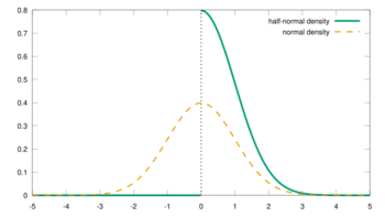
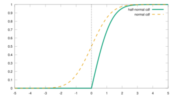
Half-normal distribution

Short description: Probability distribution

Half-normal distribution

Probability density function [math]\displaystyle{ \sigma=1 }[/math]
Cumulative distribution function [math]\displaystyle{ \sigma=1 }[/math]
Parameters	[math]\displaystyle{ \sigma\gt 0 }[/math] — (scale)
Support	[math]\displaystyle{ x\in[0,\infty) }[/math]
PDF	[math]\displaystyle{ f(x; \sigma) = \frac{\sqrt{2}}{\sigma\sqrt{\pi}}\exp \left( -\frac{x^2}{2\sigma^2} \right) \quad x\gt 0 }[/math]
CDF	[math]\displaystyle{ F(x; \sigma) = \operatorname{erf}\left(\frac{x}{\sigma\sqrt{2}}\right) }[/math]
Quantile	[math]\displaystyle{ Q(F;\sigma)=\sigma\sqrt{2}\operatorname{erf}^{-1}(F) }[/math]
Mean	[math]\displaystyle{ \frac{\sigma\sqrt{2}}{\sqrt{\pi}} }[/math]
Median	[math]\displaystyle{ \sigma\sqrt{2}\operatorname{erf}^{-1}(1/2) }[/math]
Mode	[math]\displaystyle{ 0 }[/math]
Variance	[math]\displaystyle{ \sigma^2\left(1 - \frac 2 \pi \right) }[/math]
Skewness	[math]\displaystyle{ \frac{\sqrt{2}(4-\pi)}{(\pi-2)^{3/2}} \approx 0.9952717 }[/math]
Kurtosis	[math]\displaystyle{ \frac{8(\pi-3)}{(\pi-2)^2} \approx 0.869177 }[/math]
Entropy	[math]\displaystyle{ \frac{1}{2} \log_2 \left( 2\pi e \sigma^2 \right) -1 }[/math]

In probability theory and statistics, the half-normal distribution is a special case of the folded normal distribution.

Let [math]\displaystyle{ X }[/math] follow an ordinary normal distribution, [math]\displaystyle{ N(0,\sigma^2) }[/math]. Then, [math]\displaystyle{ Y=|X| }[/math] follows a half-normal distribution. Thus, the half-normal distribution is a fold at the mean of an ordinary normal distribution with mean zero.

Properties

Using the [math]\displaystyle{ \sigma }[/math] parametrization of the normal distribution, the probability density function (PDF) of the half-normal is given by

[math]\displaystyle{ f_Y(y; \sigma) = \frac{\sqrt{2}}{\sigma\sqrt{\pi}}\exp \left( -\frac{y^2}{2\sigma^2} \right) \quad y \geq 0, }[/math]

where [math]\displaystyle{ E[Y] = \mu = \frac{\sigma\sqrt{2}}{\sqrt{\pi}} }[/math].

Alternatively using a scaled precision (inverse of the variance) parametrization (to avoid issues if [math]\displaystyle{ \sigma }[/math] is near zero), obtained by setting [math]\displaystyle{ \theta=\frac{\sqrt{\pi}}{\sigma\sqrt{2}} }[/math], the probability density function is given by

[math]\displaystyle{ f_Y(y; \theta) = \frac{2\theta}{\pi}\exp \left( -\frac{y^2\theta^2}{\pi} \right) \quad y \geq 0, }[/math]

where [math]\displaystyle{ E[Y] = \mu = \frac{1}{\theta} }[/math].

The cumulative distribution function (CDF) is given by

[math]\displaystyle{ F_Y(y; \sigma) = \int_0^y \frac{1}{\sigma}\sqrt{\frac{2}{\pi}} \, \exp \left( -\frac{x^2}{2\sigma^2} \right)\, dx }[/math]

Using the change-of-variables [math]\displaystyle{ z = x/(\sqrt{2}\sigma) }[/math], the CDF can be written as

[math]\displaystyle{ F_Y(y; \sigma) = \frac{2}{\sqrt{\pi}} \,\int_0^{y/(\sqrt{2}\sigma)}\exp \left(-z^2\right)dz = \operatorname{erf}\left(\frac{y}{\sqrt{2}\sigma}\right), }[/math]

where erf is the error function, a standard function in many mathematical software packages.

The quantile function (or inverse CDF) is written:

[math]\displaystyle{ Q(F;\sigma)=\sigma\sqrt{2} \operatorname{erf}^{-1}(F) }[/math]

where [math]\displaystyle{ 0\le F \le 1 }[/math] and [math]\displaystyle{ \operatorname{erf}^{-1} }[/math] is the inverse error function

The expectation is then given by

[math]\displaystyle{ E[Y] = \sigma \sqrt{2/\pi}, }[/math]

The variance is given by

[math]\displaystyle{ \operatorname{var}(Y) = \sigma^2\left(1 - \frac{2}{\pi}\right). }[/math]

Since this is proportional to the variance σ² of X, σ can be seen as a scale parameter of the new distribution.

The differential entropy of the half-normal distribution is exactly one bit less the differential entropy of a zero-mean normal distribution with the same second moment about 0. This can be understood intuitively since the magnitude operator reduces information by one bit (if the probability distribution at its input is even). Alternatively, since a half-normal distribution is always positive, the one bit it would take to record whether a standard normal random variable were positive (say, a 1) or negative (say, a 0) is no longer necessary. Thus,

[math]\displaystyle{ h(Y) = \frac{1}{2} \log_2 \left( \frac{\pi e \sigma^2}{2} \right) = \frac{1}{2} \log_2 \left( 2\pi e \sigma^2 \right) -1. }[/math]

Applications

The half-normal distribution is commonly utilized as a prior probability distribution for variance parameters in Bayesian inference applications.

Parameter estimation

Given numbers [math]\displaystyle{ \{x_i\}_{i=1}^n }[/math] drawn from a half-normal distribution, the unknown parameter [math]\displaystyle{ \sigma }[/math] of that distribution can be estimated by the method of maximum likelihood, giving

[math]\displaystyle{ \hat \sigma = \sqrt{\frac 1 n \sum_{i=1}^n x_i^2} }[/math]

The bias is equal to

[math]\displaystyle{ b \equiv \operatorname{E}\bigg[\;(\hat\sigma_\mathrm{mle} - \sigma)\;\bigg] = - \frac{\sigma}{4n} }[/math]

which yields the bias-corrected maximum likelihood estimator

[math]\displaystyle{ \hat{\sigma\,}^*_\text{mle} = \hat{\sigma\,}_\text{mle} - \hat{b\,}. }[/math]

Related distributions

• The distribution is a special case of the folded normal distribution with μ = 0.
• It also coincides with a zero-mean normal distribution truncated from below at zero (see truncated normal distribution)
• If Y has a half-normal distribution, then (Y/σ)² has a chi square distribution with 1 degree of freedom, i.e. Y/σ has a chi distribution with 1 degree of freedom.
• The half-normal distribution is a special case of the generalized gamma distribution with d = 1, p = 2, a = [math]\displaystyle{ \sqrt{2}\sigma }[/math].
• If Y has a half-normal distribution, Y ^-2 has a Levy distribution
• The Rayleigh distribution is a moment-tilted and scaled generalization of the half-normal distribution.
• Modified half-normal distribution with the pdf on [math]\displaystyle{ (0, \infty) }[/math] is given as [math]\displaystyle{ f(x)= \frac{2\beta^{\frac{\alpha}{2}} x^{\alpha-1} \exp(-\beta x^2+ \gamma x )}{\Psi{\left(\frac{\alpha}{2}, \frac{ \gamma}{\sqrt{\beta}}\right)}} }[/math], where [math]\displaystyle{ \Psi(\alpha,z)={}_1\Psi_1\left(\begin{matrix}\left(\alpha,\frac{1}{2}\right)\\(1,0)\end{matrix};z \right) }[/math] denotes the Fox–Wright Psi function.

See also

• Half-t distribution
• Truncated normal distribution
• Folded normal distribution
• Rectified Gaussian distribution

Further reading

• Leone, F. C.; Nelson, L. S.; Nottingham, R. B. (1961), "The folded normal distribution", Technometrics 3 (4): 543–550, doi:10.2307/1266560 

External links

• Half-Normal Distribution at MathWorld

(note that MathWorld uses the parameter [math]\displaystyle{ \theta = \frac{1}{\sigma}\sqrt {\pi/2} }[/math]

References

- ↑ Gelman, A. (2006), "Prior distributions for variance parameters in hierarchical models", Bayesian Analysis 1 (3): 515–534, doi:10.1214/06-ba117a
- ↑ Röver, C.; Bender, R.; Dias, S.; Schmid, C.H.; Schmidli, H.; Sturtz, S.; Weber, S.; Friede, T. (2021), "On weakly informative prior distributions for the heterogeneity parameter in Bayesian random-effects meta-analysis", Research Synthesis Methods 12 (4): 448–474, doi:10.1002/jrsm.1475, PMID 33486828
- ↑ Sun, Jingchao; Kong, Maiying; Pal, Subhadip (22 June 2021). "The Modified-Half-Normal distribution: Properties and an efficient sampling scheme". Communications in Statistics - Theory and Methods 52 (5): 1591–1613. doi:10.1080/03610926.2021.1934700. ISSN 0361-0926. https://www.tandfonline.com/doi/abs/10.1080/03610926.2021.1934700?journalCode=lsta20.