Imprecise Dirichlet process

In probability theory and statistics, the Dirichlet process (DP) is one of the most popular Bayesian nonparametric models. It was introduced by Thomas Ferguson as a prior over probability distributions.

A Dirichlet process [math]\displaystyle{ \mathrm{DP}\left(s,G_0\right) }[/math] is completely defined by its parameters: [math]\displaystyle{ G_0 }[/math] (the base distribution or base measure) is an arbitrary distribution and [math]\displaystyle{ s }[/math] (the concentration parameter) is a positive real number (it is often denoted as [math]\displaystyle{ \alpha }[/math]). According to the Bayesian paradigm these parameters should be chosen based on the available prior information on the domain.

The question is: how should we choose the prior parameters [math]\displaystyle{ \left(s,G_0\right) }[/math] of the DP, in particular the infinite dimensional one [math]\displaystyle{ G_0 }[/math], in case of lack of prior information?

To address this issue, the only prior that has been proposed so far is the limiting DP obtained for [math]\displaystyle{ s\rightarrow 0 }[/math], which has been introduced under the name of Bayesian bootstrap by Rubin; in fact it can be proven that the Bayesian bootstrap is asymptotically equivalent to the frequentist bootstrap introduced by Bradley Efron. The limiting Dirichlet process [math]\displaystyle{ s\rightarrow 0 }[/math] has been criticized on diverse grounds. From an a-priori point of view, the main criticism is that taking [math]\displaystyle{ s\rightarrow 0 }[/math] is far from leading to a noninformative prior. Moreover, a-posteriori, it assigns zero probability to any set that does not include the observations.

The imprecise Dirichlet process has been proposed to overcome these issues. The basic idea is to fix [math]\displaystyle{ s \gt 0 }[/math] but do not choose any precise base measure [math]\displaystyle{ G_0 }[/math].

More precisely, the imprecise Dirichlet process (IDP) is defined as follows:

[math]\displaystyle{ ~~\mathrm{IDP}:~\left\{\mathrm{DP}\left(s,G_0\right):~~G_0 \in \mathbb{P}\right\} }[/math]

where [math]\displaystyle{ \mathbb{P} }[/math] is the set of all probability measures. In other words, the IDP is the set of all Dirichlet processes (with a fixed [math]\displaystyle{ s \gt 0 }[/math]) obtained by letting the base measure [math]\displaystyle{ G_0 }[/math] to span the set of all probability measures.

Inferences with the Imprecise Dirichlet Process

Let [math]\displaystyle{ P }[/math] a probability distribution on [math]\displaystyle{ (\mathbb{X},\mathcal{B}) }[/math] (here [math]\displaystyle{ \mathbb{X} }[/math] is a standard Borel space with Borel [math]\displaystyle{ \sigma }[/math]-field [math]\displaystyle{ \mathcal{B} }[/math]) and assume that [math]\displaystyle{ P\sim \mathrm{DP}(s,G_0) }[/math]. Then consider a real-valued bounded function [math]\displaystyle{ f }[/math] defined on [math]\displaystyle{ (\mathbb{X},\mathcal{B}) }[/math]. It is well known that the expectation of [math]\displaystyle{ E[f] }[/math] with respect to the Dirichlet process is

[math]\displaystyle{ \mathcal{E} [ E(f) ]=\mathcal{E}\left[\int f \, dP\right]=\int f \,d\mathcal{E}[P] = \int f \, dG_0. }[/math]

One of the most remarkable properties of the DP priors is that the posterior distribution of [math]\displaystyle{ P }[/math] is again a DP. Let [math]\displaystyle{ X_1,\dots,X_n }[/math] be an independent and identically distributed sample from [math]\displaystyle{ P }[/math] and [math]\displaystyle{ P \sim Dp(s,G_0) }[/math], then the posterior distribution of [math]\displaystyle{ P }[/math] given the observations is

[math]\displaystyle{ P\mid X_1,\dots,X_n \sim Dp\left(s+n, G_n\right),~~~ \text{with}~~~~~~ G_n=\frac{s}{s+n} G_0+ \frac{1}{s+n} \sum\limits_{i=1}^n \delta_{X_i}, }[/math]

where [math]\displaystyle{ \delta_{X_i} }[/math] is an atomic probability measure (Dirac's delta) centered at [math]\displaystyle{ X_i }[/math]. Hence, it follows that [math]\displaystyle{ \mathcal{E}[E(f)\mid X_1,\dots,X_n]= \int f \, dG_n. }[/math] Therefore, for any fixed [math]\displaystyle{ G_0 }[/math], we can exploit the previous equations to derive prior and posterior expectations.

In the IDP [math]\displaystyle{ G_0 }[/math] can span the set of all distributions [math]\displaystyle{ \mathbb{P} }[/math]. This implies that we will get a different prior and posterior expectation of [math]\displaystyle{ E(f) }[/math] for any choice of [math]\displaystyle{ G_0 }[/math]. A way to characterize inferences for the IDP is by computing lower and upper bounds for the expectation of [math]\displaystyle{ E(f) }[/math] w.r.t. [math]\displaystyle{ G_0 \in \mathbb{P} }[/math]. A-priori these bounds are:

[math]\displaystyle{ \underline{\mathcal{E}} [E(f)]=\inf\limits_{ G_0 \in \mathbb{P}} \int f \,dG_0=\inf f, ~~~~\overline{\mathcal{E}} [E(f)]=\sup\limits_{ G_0 \in \mathbb{P}} \int f \,dG_0=\sup f, }[/math]

the lower (upper) bound is obtained by a probability measure that puts all the mass on the infimum (supremum) of [math]\displaystyle{ f }[/math], i.e., [math]\displaystyle{ G_0=\delta_{X_0} }[/math] with [math]\displaystyle{ X_0=\arg \inf f }[/math] (or respectively with [math]\displaystyle{ X_0=\arg \sup f }[/math]). From the above expressions of the lower and upper bounds, it can be observed that the range of [math]\displaystyle{ \mathcal{E}[E(f)] }[/math] under the IDP is the same as the original range of [math]\displaystyle{ f }[/math]. In other words, by specifying the IDP, we are not giving any prior information on the value of the expectation of [math]\displaystyle{ f }[/math]. A-priori, IDP is therefore a model of prior (near)-ignorance for [math]\displaystyle{ E(f) }[/math].

A-posteriori, IDP can learn from data. The posterior lower and upper bounds for the expectation of [math]\displaystyle{ E(f) }[/math] are in fact given by:

[math]\displaystyle{ \begin{align} \underline{\mathcal{E}} [E(f)\mid X_1,\dots,X_n] & = \inf\limits_{ G_0 \in \mathbb{P}} \int f \, dG_n = \frac{s}{s+n} \inf f+ \int f(X) \frac{1}{s+n} \sum\limits_{i=1}^n \delta_{X_i}(dX) \\ & =\frac{s}{s+n} \inf f+ \frac{n}{s+n} \frac{\sum\limits_{i=1}^n f(X_i)}{n},\\[6pt] \overline{\mathcal{E}} [E(f)\mid X_1,\dots,X_n]&=\sup\limits_{ G_0 \in \mathbb{P}} \int f \, dG_n= \frac{s}{s+n} \sup f+ \int f(X) \frac{1}{s+n} \sum\limits_{i=1}^n \delta_{X_i}(dX) \\ & =\frac{s}{s+n} \sup f+ \frac{n}{s+n} \frac{\sum\limits_{i=1}^n f(X_i)}{n}. \end{align} }[/math]

It can be observed that the posterior inferences do not depend on [math]\displaystyle{ G_0 }[/math]. To define the IDP, the modeler has only to choose [math]\displaystyle{ s }[/math] (the concentration parameter). This explains the meaning of the adjective near in prior near-ignorance, because the IDP requires by the modeller the elicitation of a parameter. However, this is a simple elicitation problem for a nonparametric prior, since we only have to choose the value of a positive scalar (there are not infinitely many parameters left in the IDP model).

Finally, observe that for [math]\displaystyle{ n \rightarrow \infty }[/math], IDP satisfies

[math]\displaystyle{ \underline{\mathcal{E}} \left[E(f)\mid X_1, \dots,X_n\right], \quad \overline{\mathcal{E}} \left[E(f) \mid X_1,\dots,X_n\right] \rightarrow S(f), }[/math]

where [math]\displaystyle{ S(f)=\lim_{n\rightarrow \infty} \tfrac{1}{n}\sum_{i=1}^n f(X_i) }[/math]. In other words, the IDP is consistent.

Lower (red) and Upper (blue) cumulative distribution for the observations {−1.17, 0.44, 1.17, 3.28, 1.44, 1.98}

Choice of the prior strength [math]\displaystyle{ s }[/math]

The IDP is completely specified by [math]\displaystyle{ s }[/math], which is the only parameter left in the prior model. Since the value of [math]\displaystyle{ s }[/math] determines how quickly lower and upper posterior expectations converge at the increase of the number of observations, [math]\displaystyle{ s }[/math] can be chosen so to match a certain convergence rate. The parameter [math]\displaystyle{ s }[/math] can also be chosen to have some desirable frequentist properties (e.g., credible intervals to be calibrated frequentist intervals, hypothesis tests to be calibrated for the Type I error, etc.), see Example: median test

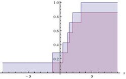
Example: estimate of the cumulative distribution

Let [math]\displaystyle{ X_1,\dots, X_n }[/math] be i.i.d. real random variables with cumulative distribution function [math]\displaystyle{ F(x) }[/math].

Since [math]\displaystyle{ F(x)=E[\mathbb{I}_{(\infty,x]}] }[/math], where [math]\displaystyle{ \mathbb{I}_{(\infty,x]} }[/math] is the indicator function, we can use IDP to derive inferences about [math]\displaystyle{ F(x). }[/math] The lower and upper posterior mean of [math]\displaystyle{ F(x) }[/math] are

[math]\displaystyle{ \begin{align} & \underline{\mathcal{E}}\left[F(x)\mid X_1,\dots,X_n\right] = \underline{\mathcal{E}} [E(\mathbb{I}_{(\infty,x]})\mid X_1,\dots,X_n] \\ = {} & \frac{n}{s+n} \frac{\sum\limits_{i=1}^n \mathbb{I}_{(\infty,x]}(X_i)}{n} =\frac{n}{s+n}\hat{F}(x), \\[12pt] & \overline{\mathcal{E}}\left[F(x)\mid X_1,\dots,X_n\right] = \overline{\mathcal{E}} \left[E(\mathbb{I}_{(\infty,x]})\mid X_1,\dots,X_n\right] \\ = {} & \frac{s}{s+n}+ \frac{n}{s+n} \frac{\sum\limits_{i=1}^n \mathbb{I}_{(\infty,x]}(X_i)}{n} = \frac{s}{s+n}+ \frac{n}{s+n} \hat{F}(x). \end{align} }[/math]

where [math]\displaystyle{ \hat{F}(x) }[/math] is the empirical distribution function. Here, to obtain the lower we have exploited the fact that [math]\displaystyle{ \inf \mathbb{I}_{(\infty,x]}=0 }[/math] and for the upper that [math]\displaystyle{ \sup \mathbb{I}_{(\infty,x]}=1 }[/math].

Beta distributions for the lower (red) and upper (blue) probability corresponding to the observations {-1.17, 0.44, 1.17, 3.28, 1.44, 1.98}. The area in [0,0.5] gives the lower (0.891) and the upper (0.9375) probability of the hypothesis "the median is greater than zero".

Note that, for any precise choice of [math]\displaystyle{ G_0 }[/math] (e.g., normal distribution [math]\displaystyle{ \mathcal{N}(x;0,1) }[/math]), the posterior expectation of [math]\displaystyle{ F(x) }[/math] will be included between the lower and upper bound.

Example: median test

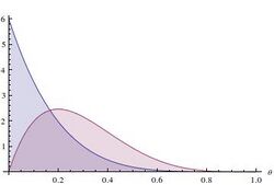
IDP can also be used for hypothesis testing, for instance to test the hypothesis [math]\displaystyle{ F(0)\lt 0.5 }[/math] , i.e., the median of [math]\displaystyle{ F }[/math] is greater than zero. By considering the partition [math]\displaystyle{ (-\infty,0],(0,\infty) }[/math] and the property of the Dirichlet process, it can be shown that the posterior distribution of [math]\displaystyle{ F(0) }[/math] is

[math]\displaystyle{ F(0) \sim \mathrm{Beta}(\alpha_0+n_{\lt 0},\beta_0+n-n_{\lt 0}) }[/math]

where [math]\displaystyle{ n_{\lt 0} }[/math] is the number of observations that are less than zero,

[math]\displaystyle{ \alpha_0=s\int_{-\infty}^0 dG_0 }[/math] and [math]\displaystyle{ \beta_0=s\int_0^\infty dG_0. }[/math]

By exploiting this property, it follows that

[math]\displaystyle{ \underline{\mathcal{P}} [F(0)\lt 0.5\mid X_1,\dots,X_n] = \int\limits_0^{0.5} \mathrm{Beta}(\theta;s+n_{\lt 0},n-n_{\lt 0})d\theta=I_{1/2}(s+n_{\lt 0},n-n_{\lt 0}), }[/math]

[math]\displaystyle{ \overline{\mathcal{P}} [F(0)\lt 0.5\mid X_1,\dots,X_n]=\int\limits_0^{0.5} \mathrm{Beta}(\theta;n_{\lt 0},s+n-n_{\lt 0})d\theta=I_{1/2}(n_{\lt 0},s+n-n_{\lt 0}). }[/math]

where [math]\displaystyle{ I_{x}(\alpha,\beta) }[/math] is the regularized incomplete beta function. We can thus perform the hypothesis test

[math]\displaystyle{ \underline{\mathcal{P}} [F(0)\lt 0.5\mid X_1,\dots,X_n]\gt 1-\gamma, ~~\overline{\mathcal{P}} [F(0)\lt 0.5\mid X_1,\dots,X_n]\gt 1-\gamma, }[/math]

(with [math]\displaystyle{ 1-\gamma=0.95 }[/math] for instance) and then

1. if both the inequalities are satisfied we can declare that [math]\displaystyle{ F(0)\lt 0.5 }[/math] with probability larger than [math]\displaystyle{ 1-\gamma }[/math];
2. if only one of the inequality is satisfied (which has necessarily to be the one for the upper), we are in an indeterminate situation, i.e., we cannot decide;
3. if both are not satisfied, we can declare that the probability that [math]\displaystyle{ F(0)\lt 0.5 }[/math] is lower than the desired probability of [math]\displaystyle{ 1-\gamma }[/math].

IDP returns an indeterminate decision when the decision is prior dependent (that is when it would depend on the choice of [math]\displaystyle{ G_0 }[/math]).

By exploiting the relationship between the cumulative distribution function of the Beta distribution, and the cumulative distribution function of a random variable Z from a binomial distribution, where the "probability of success" is p and the sample size is n:

[math]\displaystyle{ F(k;n,p) = \Pr(Z \le k) = I_{1-p}(n-k, k+1) = 1 - I_p(k+1,n-k), }[/math]

we can show that the median test derived with th IDP for any choice of [math]\displaystyle{ s\geq 1 }[/math] encompasses the one-sided frequentist sign test as a test for the median. It can in fact be verified that for [math]\displaystyle{ s= 1 }[/math] the [math]\displaystyle{ p }[/math]-value of the sign test is equal to [math]\displaystyle{ 1-\underline{\mathcal{P}} [F(0)\lt 0.5\mid X_1,\dots,X_n] }[/math]. Thus, if [math]\displaystyle{ \underline{\mathcal{P}} [F(0)\lt 0.5\mid X_1,\dots,X_n]\gt 0.95 }[/math] then the [math]\displaystyle{ p }[/math]-value is less than [math]\displaystyle{ 0.05 }[/math] and, thus, they two tests have the same power.

Applications of the Imprecise Dirichlet Process

Dirichlet processes are frequently used in Bayesian nonparametric statistics. The Imprecise Dirichlet Process can be employed instead of the Dirichlet processes in any application in which prior information is lacking (it is therefore important to model this state of prior ignorance).

In this respect, the Imprecise Dirichlet Process has been used for nonparametric hypothesis testing, see the Imprecise Dirichlet Process statistical package. Based on the Imprecise Dirichlet Process, Bayesian nonparametric near-ignorance versions of the following classical nonparametric estimators have been derived: the Wilcoxon rank sum test and the Wilcoxon signed-rank test.

A Bayesian nonparametric near-ignorance model presents several advantages with respect to a traditional approach to hypothesis testing.

1. The Bayesian approach allows us to formulate the hypothesis test as a decision problem. This means that we can verify the evidence in favor of the null hypothesis and not only rejecting it and take decisions which minimize the expected loss.
2. Because of the nonparametric prior near-ignorance, IDP based tests allows us to start the hypothesis test with very weak prior assumptions, much in the direction of letting data speak for themselves.
3. Although the IDP test shares several similarities with a standard Bayesian approach, at the same time it embodies a significant change of paradigm when it comes to take decisions. In fact the IDP based tests have the advantage of producing an indeterminate outcome when the decision is prior-dependent. In other words, the IDP test suspends the judgment when the option which minimizes the expected loss changes depending on the Dirichlet Process base measure we focus on.
4. It has been empirically verified that when the IDP test is indeterminate, the frequentist tests are virtually behaving as random guessers. This surprising result has practical consequences in hypothesis testing. Assume that we are trying to compare the effects of two medical treatments (Y is better than X) and that, given the available data, the IDP test is indeterminate. In such a situation the frequentist test always issues a determinate response (for instance I can tell that Y is better than X), but it turns out that its response is completely random, like if we were tossing of a coin. On the other side, the IDP test acknowledges the impossibility of making a decision in these cases. Thus, by saying "I do not know", the IDP test provides a richer information to the analyst. The analyst could for instance use this information to collect more data.

Categorical variables

For categorical variables, i.e., when [math]\displaystyle{ \mathbb{X} }[/math] has a finite number of elements, it is known that the Dirichlet process reduces to a Dirichlet distribution. In this case, the Imprecise Dirichlet Process reduces to the Imprecise Dirichlet model proposed by Walley as a model for prior (near)-ignorance for chances.

See also

Imprecise probability

Robust Bayesian analysis

External links

• Open source implementation of hypothesis tests based on the IDP
• The imprecise probability group at IDSIA

References

- ↑ Ferguson, Thomas (1973). "Bayesian analysis of some nonparametric problems". Annals of Statistics 1 (2): 209–230. doi:10.1214/aos/1176342360.
- ↑ 2.0 2.1 Rubin D (1981). The Bayesian bootstrap. Ann. Stat. 9 130–134
- ↑ Efron B (1979). Bootstrap methods: Another look at the jackknife. Ann. Stat. 7 1–26
- ↑ Sethuraman, J.; Tiwari, R. C. (1981). "Convergence of Dirichlet measures and the interpretation of their parameter". Defense Technical Information Center.
- ↑ Benavoli, Alessio; Mangili, Francesca; Corani, Giorgio; Ruggeri, Fabrizio; Zaffalon, Marco (2014). A Bayesian Wilcoxon signed-rank test based on the Dirichlet process. Proceedings of the 30th International Conference on Machine Learning (ICML 2014).
- ↑ Walley, Peter (1991). Statistical Reasoning with Imprecise Probabilities. London: Chapman and Hall. ISBN 0-412-28660-2.