Kumaraswamy distribution

Kumaraswamy

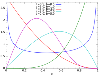
Probability density function
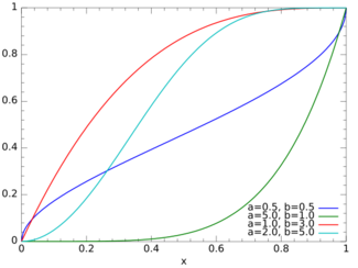
Cumulative distribution function
Parameters	[math]\displaystyle{ a\gt 0\, }[/math] (real) [math]\displaystyle{ b\gt 0\, }[/math] (real)
Support	[math]\displaystyle{ x \in (0,1)\, }[/math]
PDF	[math]\displaystyle{ abx^{a-1}(1-x^a)^{b-1}\, }[/math]
CDF	[math]\displaystyle{ 1-(1-x^a)^b }[/math]
Mean	[math]\displaystyle{ \frac{b\Gamma(1+\tfrac{1}{a})\Gamma(b)}{\Gamma(1+\tfrac{1}{a}+b)}\, }[/math]
Median	[math]\displaystyle{ \left(1-2^{-1/b}\right)^{1/a} }[/math]
Mode	[math]\displaystyle{ \left(\frac{a-1}{ab-1}\right)^{1/a} }[/math] for [math]\displaystyle{ a\geq 1, b\geq 1, (a,b)\neq (1,1) }[/math]
Variance	(complicated-see text)
Skewness	(complicated-see text)
Kurtosis	(complicated-see text)
Entropy	[math]\displaystyle{ \left(1\!-\!\tfrac{1}{b}\right)+\left(1\!-\!\tfrac{1}{a}\right)H_b-\ln(ab) }[/math]

In probability and statistics, the Kumaraswamy's double bounded distribution is a family of continuous probability distributions defined on the interval (0,1). It is similar to the beta distribution, but much simpler to use especially in simulation studies since its probability density function, cumulative distribution function and quantile functions can be expressed in closed form. This distribution was originally proposed by Poondi Kumaraswamy for variables that are lower and upper bounded with a zero-inflation. This was extended to inflations at both extremes [0,1] in later work with S. G . Fletcher.

Characterization

Probability density function

The probability density function of the Kumaraswamy distribution without considering any inflation is

[math]\displaystyle{ f(x; a,b) = a b x^{a-1}{ (1-x^a)}^{b-1}, \ \ \mbox{where} \ \ x \in (0,1), }[/math]

and where a and b are non-negative shape parameters.

Cumulative distribution function

The cumulative distribution function is

[math]\displaystyle{ F(x; a,b)=\int_{0}^{x}f(\xi; a,b) d\xi = 1-(1-x^a)^b.\ }[/math]

Quantile function

The inverse cumulative distribution function (quantile function) is

[math]\displaystyle{ F^{-1}(y; a,b)=(1-(1-y)^\frac{1}{b})^\frac{1}{a}. \ }[/math]

Generalizing to arbitrary interval support

In its simplest form, the distribution has a support of (0,1). In a more general form, the normalized variable x is replaced with the unshifted and unscaled variable z where:

[math]\displaystyle{ x = \frac{z-z_{\text{min}}}{z_{\text{max}}-z_{\text{min}}} , \qquad z_{\text{min}} \le z \le z_{\text{max}}. \,\! }[/math]

Properties

The raw moments of the Kumaraswamy distribution are given by:

[math]\displaystyle{ m_n = \frac{b\Gamma(1+n/a)\Gamma(b)}{\Gamma(1+b+n/a)} = bB(1+n/a,b)\, }[/math]

where B is the Beta function and Γ(.) denotes the Gamma function. The variance, skewness, and excess kurtosis can be calculated from these raw moments. For example, the variance is:

[math]\displaystyle{ \sigma^2=m_2-m_1^2. }[/math]

The Shannon entropy (in nats) of the distribution is:

[math]\displaystyle{ H=\left(1\!-\!\tfrac{1}{a}\right)+\left(1\!-\!\tfrac{1}{b}\right)H_b-\ln(ab) }[/math]

where [math]\displaystyle{ H_i }[/math] is the harmonic number function.

Relation to the Beta distribution

The Kumaraswamy distribution is closely related to Beta distribution. Assume that X_a,b is a Kumaraswamy distributed random variable with parameters a and b. Then X_a,b is the a-th root of a suitably defined Beta distributed random variable. More formally, Let Y_1,b denote a Beta distributed random variable with parameters [math]\displaystyle{ \alpha=1 }[/math] and [math]\displaystyle{ \beta=b }[/math]. One has the following relation between X_a,b and Y_1,b.

[math]\displaystyle{ X_{a,b}=Y^{1/a}_{1,b}, }[/math]

with equality in distribution.

[math]\displaystyle{ \operatorname{P}\{X_{a,b}\le x\}=\int_0^x ab t^{a-1}(1-t^a)^{b-1}dt= \int_0^{x^a} b(1-t)^{b-1}dt=\operatorname{P}\{Y_{1,b}\le x^a\} =\operatorname{P}\{Y^{1/a}_{1,b}\le x\} . }[/math]

One may introduce generalised Kumaraswamy distributions by considering random variables of the form [math]\displaystyle{ Y^{1/\gamma}_{\alpha,\beta} }[/math], with [math]\displaystyle{ \gamma\gt 0 }[/math] and where [math]\displaystyle{ Y_{\alpha,\beta} }[/math] denotes a Beta distributed random variable with parameters [math]\displaystyle{ \alpha }[/math] and [math]\displaystyle{ \beta }[/math]. The raw moments of this generalized Kumaraswamy distribution are given by:

[math]\displaystyle{ m_n = \frac{\Gamma(\alpha+\beta)\Gamma(\alpha+n/\gamma)}{\Gamma(\alpha)\Gamma(\alpha+\beta+n/\gamma)}. }[/math]

Note that we can re-obtain the original moments setting [math]\displaystyle{ \alpha=1 }[/math], [math]\displaystyle{ \beta=b }[/math] and [math]\displaystyle{ \gamma=a }[/math]. However, in general, the cumulative distribution function does not have a closed form solution.

Related distributions

• If [math]\displaystyle{ X \sim \textrm{Kumaraswamy}(1,1)\, }[/math] then [math]\displaystyle{ X \sim U(0,1)\, }[/math] (Uniform distribution)
• If [math]\displaystyle{ X \sim U(0,1) \, }[/math] then [math]\displaystyle{ {\left( 1-X^{\tfrac{1}{b}} \right)}^{ \tfrac{1}{a}} \sim \textrm{Kumaraswamy}(a,b) \, }[/math]
• If [math]\displaystyle{ X \sim \textrm{Beta}(1,b) \, }[/math] (Beta distribution) then [math]\displaystyle{ X \sim \textrm{Kumaraswamy}(1,b)\, }[/math]
• If [math]\displaystyle{ X \sim \textrm{Beta}(a,1) \, }[/math] (Beta distribution) then [math]\displaystyle{ X \sim \textrm{Kumaraswamy}(a,1)\, }[/math]
• If [math]\displaystyle{ X \sim \textrm{Kumaraswamy}(a,1)\, }[/math] then [math]\displaystyle{ (1-X) \sim \textrm{Kumaraswamy}(1, a)\, }[/math]
• If [math]\displaystyle{ X \sim \textrm{Kumaraswamy}(1,a)\, }[/math] then [math]\displaystyle{ (1-X) \sim \textrm{Kumaraswamy}(a, 1)\, }[/math]
• If [math]\displaystyle{ X \sim \textrm{Kumaraswamy}(a,1)\, }[/math] then [math]\displaystyle{ -\log(X) \sim \textrm{Exponential}(a)\, }[/math]
• If [math]\displaystyle{ X \sim \textrm{Kumaraswamy}(1,b)\, }[/math] then [math]\displaystyle{ -\log(1-X) \sim \textrm{Exponential}(b)\, }[/math]
• If [math]\displaystyle{ X \sim \textrm{Kumaraswamy}(a,b)\, }[/math] then [math]\displaystyle{ X \sim \textrm{GB1}(a, 1, 1, b)\, }[/math], the generalized beta distribution of the first kind.

Example

An example of the use of the Kumaraswamy distribution is the storage volume of a reservoir of capacity z whose upper bound is z_max and lower bound is 0, which is also a natural example for having two inflations as many reservoirs have nonzero probabilities for both empty and full reservoir states.

References

- ↑ Kumaraswamy, P. (1980). "A generalized probability density function for double-bounded random processes". Journal of Hydrology 46 (1–2): 79–88. doi:10.1016/0022-1694(80)90036-0. ISSN 0022-1694. Bibcode: 1980JHyd...46...79K.
- ↑ 2.0 2.1 Fletcher, S.G.; Ponnambalam, K. (1996). "Estimation of reservoir yield and storage distribution using moments analysis". Journal of Hydrology 182 (1–4): 259–275. doi:10.1016/0022-1694(95)02946-x. ISSN 0022-1694. Bibcode: 1996JHyd..182..259F.
- ↑ Lemonte, Artur J. (2011). "Improved point estimation for the Kumaraswamy distribution". Journal of Statistical Computation and Simulation 81 (12): 1971–1982. doi:10.1080/00949655.2010.511621. ISSN 0094-9655.
- ↑ CRIBARI-NETO, FRANCISCO; SANTOS, JÉSSICA (2019). "Inflated Kumaraswamy distributions". Anais da Academia Brasileira de Ciências 91 (2). doi:10.1590/0001-3765201920180955. ISSN 1678-2690. PMID 31141016. http://pdfs.semanticscholar.org/74cf/6193ee129558fb0f7d03835852e1cdd72452.pdf.
- ↑ Michalowicz, Joseph Victor; Nichols, Jonathan M.; Bucholtz, Frank (2013). Handbook of Differential Entropy. Chapman and Hall/CRC. p. 100. ISBN 978-1-4665-8317-7.
- ↑ 6.0 6.1 Jones, M.C. (2009). "Kumaraswamy's distribution: A beta-type distribution with some tractability advantages". Statistical Methodology 6 (1): 70–81. doi:10.1016/j.stamet.2008.04.001. ISSN 1572-3127.