Line integral convolution

In scientific visualization, line integral convolution (LIC) is a method to visualize a vector field (such as fluid motion) at high spatial resolutions.[1] The LIC technique was first proposed by Brian Cabral and Leith Casey Leedom in 1993.[2]
In LIC, discrete numerical line integration is performed along the field lines (curves) of the vector field on a uniform grid. The integral operation is a convolution of a filter kernel and an input texture, often white noise.[1] In signal processing, this process is known as a discrete convolution.[3]
Overview
Traditional visualizations of vector fields use small arrows or lines to represent vector direction and magnitude. This method has a low spatial resolution, which limits the density of presentable data and risks obscuring characteristic features in the data.[1][3] More sophisticated methods, such as streamlines and particle tracing techniques, can be more revealing but are highly dependent on proper seed points.[1] Texture-based methods, like LIC, avoid these problems since they depict the entire vector field at point-like (pixel) resolution.[1]
In user testing, LIC was found to be particularly good for identifying critical points.[4]
Algorithm
Informal description
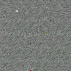
LIC causes output values to be strongly correlated along the field lines, but uncorrelated in orthogonal directions.[1] As a result, the field lines contrast each other and stand out visually from the background.
Intuitively, the process can be understood with the following example: the flow of a vector field can be visualized by overlaying a fixed, random pattern of dark and light paint. As the flow passes by the paint, the fluid picks up some of the paint's color, averaging it with the color it has already acquired. The result is a randomly striped, smeared texture where points along the same streamline tend to have a similar color. Other physical examples include:
- whorl patterns of paint, oil, or foam on a river
- fine sand being blown by strong wind[5]
Formal mathematical description
Although the input vector field and the result image are discretized, it pays to look at it from a continuous viewpoint.[1] Let be the vector field given in some domain . Although the input vector field is typically discretized, we regard the field as defined in every point of , i.e. we assume an interpolation. Streamlines, or more generally field lines, are tangent to the vector field in each point. They end either at the boundary of or at critical points where . For the sake of simplicity, critical points and boundaries are ignored in the following.
A field line , parametrized by arc length , is defined as
Let be the field line that passes through the point for . Then the image gray value at is set to
where is the convolution kernel, is the noise image, and is the length of field line segment that is followed.
has to be computed for each pixel in the LIC image. If carried out naively, this is quite expensive. First, the field lines have to be computed using a numerical method for solving ordinary differential equations, like a Runge–Kutta method, and then for each pixel the convolution along a field line segment has to be calculated.
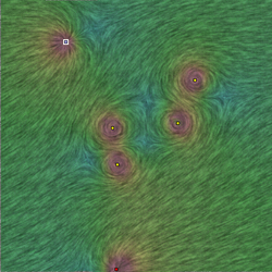
The final image will normally be colored in some way. Typically, some scalar field in (like the vector length) is used to determine the hue, while the grayscale LIC output determines the brightness.
Different choices of convolution kernels and random noise produce different textures; for example, pink noise produces a cloudy pattern where areas of higher flow stand out as smearing, suitable for weather visualization. Further refinements in the convolution can improve the quality of the image.[6]
Programming description
Algorithmically, LIC takes a vector field and noise texture as input, and outputs a texture. The process starts by generating in the domain of the vector field a random gray level image at the desired output resolution. Then, for every pixel in this image, the forward and backward streamline of a fixed arc length is calculated. The value assigned to the current pixel is computed by a convolution of a suitable convolution kernel with the gray levels of all the noise pixels lying on a segment of this streamline. This creates a gray level LIC image.
Versions
Basic

Basic LIC images are grayscale images, without color and animation. While such LIC images convey the direction of the field vectors, they do not indicate orientation; for stationary fields, this can be remedied by animation. Basic LIC images do not show the length of the vectors (or the strength of the field).
Color

The length of the vectors (or the strength of the field) is usually coded in color; alternatively, animation can be used.[2][1]
Animation

Top: normal box filter (average).
Middle: sinusoidal filter at .
Bottom: sinusoidal filter at .
LIC images can be animated by using a kernel that changes over time. Samples at a constant time from the streamline would still be used, but instead of averaging all pixels in a streamline with a static kernel, a ripple-like kernel constructed from a periodic function multiplied by a Hann function acting as a window (in order to prevent artifacts) is used. The periodic function is then shifted along the period to create an animation.
Fast LIC (FLIC)
The computation can be significantly accelerated by re-using parts of already computed field lines, specializing to a box function as convolution kernel and avoiding redundant computations during convolution.[1] The resulting fast LIC method can be generalized to convolution kernels that are arbitrary polynomials.[7]
Oriented Line Integral Convolution (OLIC)
Because LIC does not encode flow orientation, it cannot distinguish between streamlines of equal direction but opposite orientation.[8] Oriented Line Integral Convolution (OLIC) solves this issue by using a ramp-like asymmetric kernel and a low-density noise texture.[8] The kernel asymmetrically modulates the intensity along the streamline, producing a trace that encodes orientation; the low-density of the noise texture prevents smeared traces from overlapping, aiding readability.
Fast Rendering of Oriented Line Integral Convolution (FROLIC) is a variation that approximates OLIC by rendering each trace in discrete steps instead of as a continuous smear.[8][9]
Unsteady Flow LIC (UFLIC)
For time-dependent vector fields (unsteady flow), a variant called Unsteady Flow LIC has been designed that maintains the coherence of the flow animation.[10] An interactive GPU-based implementation of UFLIC has been presented.[11]
Parallel
Since the computation of an LIC image is expensive but inherently parallel, the process has been parallelized[12] and, with availability of GPU-based implementations, interactive on PCs.
Multidimensional
Note that the domain does not have to be a 2D domain: the method is applicable to higher dimensional domains using multidimensional noise fields. However, the visualization of the higher-dimensional LIC texture is problematic; one way is to use interactive exploration with 2D slices that are manually positioned and rotated. The domain does not have to be flat either; the LIC texture can be computed also for arbitrarily shaped 2D surfaces in 3D space.[13]
Applications
This technique has been applied to a wide range of problems since it first was published in 1993, both scientific and creative, including:
Representing vector fields:
- visualization of steady (time-independent) flows (streamlines)[14]
- visual exploration of 2D autonomous dynamical systems[15]
- wind mapping[16]
- water flow mapping
Artistic effects for image generation and stylization:
- pencil drawing[17] (automatic pencil drawing generation technique using LIC pencil filter[18])
- automatic generation of hair textures[19]
- creating marbling texture[20]
Terrain generalization:
- creating generalized shaded relief[21]
Implementations
- GPU Based Image Processing Tools by Raymond McGuire
- ParaView : Line Integral Convolution
- A 2D flow visualization tool based on LIC and RK4. Developed using C++ and VTK. by Andres Bejarano
- Wolfram Research (2008), LineIntegralConvolutionPlot, Wolfram Language function, https://reference.wolfram.com/language/ref/LineIntegralConvolutionPlot.html (updated 2014).
See also
References
- ↑ 1.0 1.1 1.2 1.3 1.4 1.5 1.6 1.7 1.8 Stalling, Detlev; Hege, Hans-Christian (August 6–11, 1995). "Fast and Resolution Independent Line Integral Convolution". SIGGRAPH '95. Los Angeles, California. pp. 249–256. doi:10.1145/218380.218448. ISBN 0-89791-701-4. https://archive.org/details/computergraphics00sigg/page/249.
- ↑ 2.0 2.1 Cabral, Brian; Leedom, Leith Casey (August 2–6, 1993). "Imaging Vector Fields Using Line Integral Convolution". SIGGRAPH '93. Anaheim, California. pp. 263–270. doi:10.1145/166117.166151. ISBN 0-89791-601-8.
- ↑ 3.0 3.1 Ward, Matthew O. (February 5, 1996). "Line Integral Convolution for Flow Visualization". https://web.cs.wpi.edu/~matt/courses/cs563/talks/flowvis/lic.html.
- ↑ Laidlaw, David H.; Kirby, Robert M.; Davidson, J. Scott; Miller, Timothy S.; da Silva, Marco; Warren, William H.; Tarr, Michael J. (October 21–26, 2001). "Quantitative Comparative Evaluation of 2D Vector Field Visualization Methods". San Diego, CA, USA. pp. 143–150.
- ↑ Liu, Zhanping (Aug 21, 2007). "LIC (Line Integral Convolution)". http://www.zhanpingliu.org/research/flowvis/LIC/LIC.htm.
- ↑ Weiskopf, Daniel (2009). "Iterative Twofold Line Integral Convolution for Texture-Based Vector Field Visualization". in Möller, Torsten; Hamann, Bernd; Russell, Robert D.. Mathematical Foundations of Scientific Visualization, Computer Graphics, and Massive Data Exploration. Mathematics and Visualization. Berlin, New York: Springer. pp. 191–211. doi:10.1007/b106657_10. ISBN 978-3-540-25076-0. https://scholar.archive.org/work/t3e74cfmmjg6zcotlqqzy5dihq.
- ↑ Hege, Hans-Christian; Stalling, Detlev (1998), "Fast LIC with Piecewise Polynomial Filter Kernels", in Hege, Hans-Christian; Polthier, Konrad, Mathematical Visualization, Berlin, Heidelberg: Springer-Verlag, pp. 295–314, doi:10.1007/978-3-662-03567-2_22, ISBN 978-3-642-08373-0
- ↑ 8.0 8.1 8.2 Wegenkittl, Rainer; Gröller, Eduard (24 October 1997). "Fast oriented line integral convolution for vector field visualization via the Internet". Proceedings. Visualization '97 (Cat. No. 97CB36155). pp. 309–316. doi:10.1109/VISUAL.1997.663897. ISBN 0-8186-8262-0. https://www.cg.tuwien.ac.at/research/vis/dynsys/frolic/frolic_crc.pdf.
- ↑ Java Exploration Tool for Dynamical Systems by R. Wegenkittl and E. Gröller.
- ↑ Shen, Han-Wei; Kam, David L. (1998). "A New Line Integral Convolution Algorithm for Visualizing Time-Varying Flow Fields". IEEE Trans Vis Comput Graph (Los Alamitos: IEEE) 4 (2): 98–108. doi:10.1109/2945.694952. ISSN 1077-2626. Bibcode: 1998ITVCG...4...98H. http://web.cse.ohio-state.edu/~shen.94/Research/Gravity/Project_2_files/Shen1998a.pdf.
- ↑ Ding, Zi'ang; Liu, Zhanping; Yu, Yang; Chen, Wei (2015). "Parallel unsteady flow line integral convolution for high-performance dense visualization". Hangzhou, China. pp. 25–30.
- ↑ Zöckler, Malte; Stalling, Detlev; Hege, Hans-Christian (1997). "Parallel Line Integral Convolution". Parallel Computing (Amsterdam: North Holland) 23 (7): 975–989. doi:10.1016/S0167-8191(97)00039-2. ISSN 0167-8191. http://www.zib.de/visual-publications/sources/src-1996/parLIC.pdf.
- ↑ Battke, Henrik; Stalling, Detlev; Hege, Hans-Christian (1997). "Fast Line Integral Convolution for Arbitrary Surfaces in 3D". in Hege, Hans-Christian; Polthier, Konrad. Visualization and Mathematics: Experiments, Simulations, and Environments. Berlin, New York: Springer. pp. 181–195. doi:10.1007/978-3-642-59195-2_12. ISBN 3-540-61269-6. https://archive.org/details/visualizationmat00fran.
- ↑ DAAC: Line Integral Convolution
- ↑ Visual exploration of 2D autonomous dynamical systems Thomas Müller2,1 and Filip Sadlo1 Published 26 February 2015 • © 2015 IOP Publishing Ltd European Journal of Physics, Volume 36, Number 3
- ↑ A real-time map of the wind in the U.S. by Fernanda Viégas and Martin Wattenberg.
- ↑ researchgate publication: Sun, Shuo & Huang, Dongwei. (2022). Efficient Region-Based Pencil Drawing.
- ↑ S. Yamamoto, Xiaoyang Mo and A. Imamiya, "Enhanced LIC pencil filter," Proceedings. International Conference on Computer Graphics, Imaging and Visualization, 2004. CGIV 2004., 2004, pp. 251-256, doi: 10.1109/CGIV.2004.1323994.
- ↑ Xiaoyang Mao, M. Kikukawa, K. Kashio and A. Imamiya, "Automatic generation of hair texture with line integral convolution," 2000 IEEE Conference on Information Visualization. An International Conference on Computer Visualization and Graphics, 2000, pp. 303-308, doi: 10.1109/IV.2000.859772.
- ↑ Xiaoyang Mao, Toshikazu Suzuki, and Atsumi Imamiya. 2003. AtelierM: a physically based interactive system for creating traditional marbling textures. In Proceedings of the 1st international conference on Computer graphics and interactive techniques in Australasia and South East Asia (GRAPHITE '03). Association for Computing Machinery, New York, NY, USA, 79–ff. https://doi.org/10.1145/604471.604489
- ↑ Bernhard Jenny (2021) Terrain generalization with line integral convolution, Cartography and Geographic Information Science, 48:1, 78-92, DOI: 10.1080/15230406.2020.1833762
| Wikibooks has a book on the topic of: Fractals/Mathematics/LIC |
 |
