Physics:Polymer scattering

Polymer scattering experiments are one of the main scientific methods used in chemistry, physics and other sciences to study the characteristics of polymeric systems: solutions, gels, compounds and more. As in most scattering experiments, it involves subjecting a polymeric sample to incident particles (with defined wavelengths), and studying the characteristics of the scattered particles: angular distribution, intensity polarization and so on. This method is quite simple and straightforward, and does not require special manipulations of the samples which may alter their properties, and hence compromise exact results. As opposed to crystallographic scattering experiments, where the scatterer or "target" has very distinct order, which leads to well defined patterns (presenting Bragg peaks for example), the stochastic nature of polymer configurations and deformations (especially in a solution), gives rise to quite different results.

Formalism

We consider a polymer as a chain of monomers, each with its position vector [math]\displaystyle{ \vec{R_i} }[/math] and scattering amplitude [math]\displaystyle{ a_i }[/math]. For simplicity, it is worthwhile considering identical monomers in the chain, such that all [math]\displaystyle{ a_i=a }[/math].

An incoming ray (of light/neutrons/X-ray etc.) has a wave vector (or momentum) [math]\displaystyle{ \vec{k}_{incident} }[/math], and is scattered by the polymer to the vector [math]\displaystyle{ \vec{k}_{final} }[/math]. This enables us to define the scattering vector [math]\displaystyle{ \vec{k}\equiv\vec{k}_{final}-\vec{k}_{incident} }[/math].

The scattering geometry: scattering of a vector [math]\displaystyle{ \vec{k}_{incident} }[/math] into [math]\displaystyle{ \vec{k}_{final} }[/math].

By coherently summing the contributions of all [math]\displaystyle{ N }[/math] monomers, we get the scattering intensity from a single polymer, as a function of [math]\displaystyle{ \vec{k} }[/math]:

[math]\displaystyle{ I(\vec{k})=|a|^2\sum_{i,j=1}^N e^{i\vec{k}\cdot(\vec{R}_i-\vec{R}_j)} }[/math]

Dilute solutions

A dilute solution of a certain polymer has a unique feature: all polymers are considered independent from each other, so that interactions between polymers may be neglected. By illuminating such a solution with a ray of considerable width, a macroscopic number of chain conformations are being sampled simultaneously. In this situation the accessible observables are all ensemble averages, i.e. averages over all possible configurations and deformations of the polymer.

In such a solution, where the polymer density is low (dilute) enough, homogenous and isotropic (on average), intermolecular contributions to the structure factor are averaged out, and only the single-molecule/polymer structure factor is preserved:

[math]\displaystyle{ S(\vec{k})=\frac1{N^2}\langle \sum_{i,j=1}^N e^{i\vec{k}\cdot(\vec{R}_i-\vec{R}_j)}\rangle }[/math]

with [math]\displaystyle{ \langle \cdot\rangle }[/math] representing the ensemble average. This reduces to the following for an isotropic system (which is typically the case):

[math]\displaystyle{ S(\vec{k})=\frac1{N^2}\langle \sum_{i,j=1}^N \frac{\sin kR_{ij}}{kR_{ij}} \rangle }[/math]

where two more definitions were made: [math]\displaystyle{ k\equiv|\vec k| }[/math] and [math]\displaystyle{ R_{ij}\equiv|\vec R_i-\vec R_j| }[/math].

Ideal chains – Debye function

A comparison between the Debye function (black) and the approximated Lorentzian (blue). One sees no major differences between them.

If the polymers of interest are ideal gaussian chains (or freely-jointed chains), in the limit of very long chains (allows performing a sort of "continuum transition"), the calculation of the structure can be carried out explicitly and result in a sort of Debye function:

[math]\displaystyle{ S_D(\vec{k})=\frac2{(kR_g)^4}[(kR_g)^2-1+e^{-(kR_g)^2}] }[/math]

With [math]\displaystyle{ R_g }[/math] being the polymer's radius of gyration.

in many practical scenarios, the above formula is approximated by the (much more convenient) Lorentzian:

[math]\displaystyle{ S_D(\vec{k})\approx\frac1{1+\frac12(kR_g)^2} }[/math]

which has a relative error of no more than 15% compared to the exact expression.

Small-angle scattering from polymers

The calculation of the structure factor for cases differing from ideal polymer chains can be quite cumbersome, and sometimes impossible to complete analytically. However, when the small-angle scattering condition is met, [math]\displaystyle{ kR_g\ll1 }[/math], the sinc term can be expanded so one gets:

[math]\displaystyle{ S(\vec{k})\approx\frac1{N^2}\langle \sum_{i,j=1}^N 1-\frac16(kR_{ij})^2 \rangle }[/math]

A Guinier plot made with X-ray scattering in the small-angle regime. The slopes of these linear curves correspond to the radius of gyration of the polymers in the solution, while different curves correspond to different concentrations.

and by utilising the definition of the radius of gyration:

[math]\displaystyle{ S(\vec{k})\approx1-\frac13(kR_{g})^2\approx e^{-\frac13(kR_{g})^2} }[/math]

where the final transition utilises once again the small-angle approximation.

We can thus approximate the scattering intensity in the small-angle regime as:

[math]\displaystyle{ \log I(k)=-\frac13k^2R_g^2+const. }[/math]

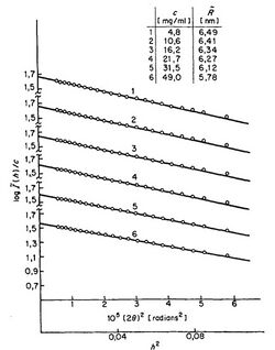
and by plotting [math]\displaystyle{ \log I(k) }[/math] vs. [math]\displaystyle{ k^2 }[/math] , a so-called "Guinier plot", we may determine the radius of gyration from the slope of this linear curve. This measure is one of many examples of how scattering experiments of polymers can reveal basic properties of those polymer chains.

Practical considerations

In order to reap the benefits of working in this small-angle regime, one must take into consideration:

• The characteristic length scale of the polymer, e.g. [math]\displaystyle{ R_g }[/math]
• The wavelength of the scattered particles

The ratio [math]\displaystyle{ \frac {R_g}{\lambda} }[/math] will determine the available angular spectrum of this regime. To see this one may consider the case of elastic scattering (even approximately elastic ). If the scattering angle is [math]\displaystyle{ \theta }[/math], we may express [math]\displaystyle{ k }[/math] as:

[math]\displaystyle{ k=\frac{4\pi}{\lambda} \sin{\frac\theta2} }[/math]

so the small-angle condition becomes [math]\displaystyle{ \frac{R_g}{\lambda} \sin{\frac\theta2}\ll1 }[/math], determining the relevant angles.

(a) Small-angle neutron scattering (SANS) and light scattering (LS) profiles of PNIPA gels and solution and (b) schematic representation of the gel network.

Example

- For visible light, [math]\displaystyle{ \lambda\sim5000 \overset{o}{A} }[/math]

- For neutrons, [math]\displaystyle{ \lambda\sim3 \overset{o}{A} }[/math]

- For "hard" X-rays, [math]\displaystyle{ \lambda\sim1 \overset{o}{A} }[/math]

while typical [math]\displaystyle{ R_g }[/math] values for polymers range in [math]\displaystyle{ 10-100 \overset{o}{A} }[/math]. This makes small-angle measurements in neutrons and X-rays a bit more tedious, as very small angles are needed, and the data in those angles is often "overpowered" by the [math]\displaystyle{ \theta=0 }[/math] spot emerging in usual scattering experiments. The problem is mitigated by conducting longer experiments with more exposure time, which allows the required data to "intensify". One must take care though, as to not allow the prolonged exposure to high levels of radiation damage the polymers (which might be a real problem when considering biological polymer samples – proteins, for example).

On the other hand, to resolve smaller polymers and structurals subtleties, one cannot always resort to using the long-wavelength rays, as the diffraction limit comes into play.

Applications

The change in the small-angle scattering signatures when the interactions between polymers are tuned. From left to right there is an increase in the amount of Magnesium in the solution, which alleviates the coulomb repulsion (thus reducing the order).

The main purpose of such scattering experiments involving polymers is to study unique properties of the sample of interest:

1. Determine the polymers "size" - radius of gyration.
2. Evaluating the structural and thermo-statistical behavior of a polymer, i.e. freely-jointed chain / freely-rotating chain etc.
3. Explore the distribution of the polymers in the sample - is it truly isotropic? Or does it favor certain directions on average?
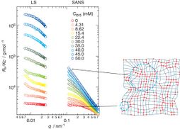
4. Identifying deformations in the polymer samples and quantifying them.
5. Examining complex interactions of polymers in the solution - between themselves, and between them and the solution. Such interactions may arise if the polymers are charged, corresponding to ionic interactions, This would have a significant impact on the particles behavior, and will result in a significant scattering signature.
6. Studying a myriad of biological substances (e.g. DNA) that are often suspended in an aqueous solution.

Further reading

• Polymers
• Static light scattering
• Biological small-angle scattering
• Neutron scattering
• Polymer characterization
• Wide-angle X-ray scattering

References

- ↑ 1.0 1.1 Doi, M.; Edwards, S.F.. The Theory of Polymer Dynamics. pp. 21–23.
- ↑ Nakanishi, Ryosuke; Machida, Ginpei; Kinoshita, Masaki; Sakurai, Kazuo; Akiba, Isamu (16 March 2016). "Anomalous small-angle X-ray scattering study on the spatial distribution of hydrophobic molecules in polymer micelles". Polymer Journal 48 (7): 801–806. doi:10.1038/pj.2016.32.
- ↑ Shibayama, Mitsuhiro (17 November 2010). "Small-angle neutron scattering on polymer gels: phase behavior, inhomogeneities and deformation mechanisms". Polymer Journal 43: 18–34. doi:10.1038/pj.2010.110.
- ↑ Pollack, Lois (2011-01-01). "SAXS Studies of Ion–Nucleic Acid Interactions". Annual Review of Biophysics 40 (1): 225–242. doi:10.1146/annurev-biophys-042910-155349. PMID 21332357.