Physics:Vertex model
A vertex model is a type of statistical mechanics model in which the Boltzmann weights are associated with a vertex in the model (representing an atom or particle).[1][2] This contrasts with a nearest-neighbour model, such as the Ising model, in which the energy, and thus the Boltzmann weight of a statistical microstate is attributed to the bonds connecting two neighbouring particles. The energy associated with a vertex in the lattice of particles is thus dependent on the state of the bonds which connect it to adjacent vertices. It turns out that every solution of the Yang–Baxter equation with spectral parameters in a tensor product of vector spaces yields an exactly-solvable vertex model.

Although the model can be applied to various geometries in any number of dimensions, with any number of possible states for a given bond, the most fundamental examples occur for two dimensional lattices, the simplest being a square lattice where each bond has two possible states. In this model, every particle is connected to four other particles, and each of the four bonds adjacent to the particle has two possible states, indicated by the direction of an arrow on the bond. In this model, each vertex can adopt
possible configurations. The energy for a given vertex can be given by
,

with a state of the lattice is an assignment of a state of each bond, with the total energy of the state being the sum of the vertex energies. As the energy is often divergent for an infinite lattice, the model is studied for a finite lattice as the lattice approaches infinite size. Periodic or domain wall[3] boundary conditions may be imposed on the model.
Discussion
For a given state of the lattice, the Boltzmann weight can be written as the product over the vertices of the Boltzmann weights of the corresponding vertex states
where the Boltzmann weights for the vertices are written
- ,
and the i, j, k, l range over the possible statuses of each of the four edges attached to the vertex. The vertex states of adjacent vertices must satisfy compatibility conditions along the connecting edges (bonds) in order for the state to be admissible.
The probability of the system being in any given state at a particular time, and hence the properties of the system are determined by the partition function, for which an analytic form is desired.
where β = 1/kT, T is temperature and k is the Boltzmann constant. The probability that the system is in any given state (microstate) is given by
so that the average value of the energy of the system is given by
In order to evaluate the partition function, firstly examine the states of a row of vertices.

The external edges are free variables, with summation over the internal bonds. Hence, form the row partition function
This can be reformulated in terms of an auxiliary n-dimensional vector space V, with a basis , and as
and as
thereby implying that T can be written as
where the indices indicate the factors of the tensor product on which R operates. Summing over the states of the bonds in the first row with the periodic boundary conditions , gives
where is the row-transfer matrix.

By summing the contributions over two rows, the result is
which upon summation over the vertical bonds connecting the first two rows gives: for M rows, this gives
and then applying the periodic boundary conditions to the vertical columns, the partition function can be expressed in terms of the transfer matrix as
where is the largest eigenvalue of . The approximation follows from the fact that the eigenvalues of are the eigenvalues of to the power of M, and as , the power of the largest eigenvalue becomes much larger than the others. As the trace is the sum of the eigenvalues, the problem of calculating reduces to the problem of finding the maximum eigenvalue of . This in itself is another field of study. However, a standard approach to the problem of finding the largest eigenvalue of is to find a large family of operators which commute with . This implies that the eigenspaces are common, and restricts the possible space of solutions. Such a family of commuting operators is usually found by means of the Yang–Baxter equation, which thus relates statistical mechanics to the study of quantum groups.
Integrability
Definition: A vertex model is integrable if, such that
This is a parameterized version of the Yang–Baxter equation, corresponding to the possible dependence of the vertex energies, and hence the Boltzmann weights R on external parameters, such as temperature, external fields, etc.
The integrability condition implies the following relation.
Proposition: For an integrable vertex model, with and defined as above, then
as endomorphisms of , where acts on the first two vectors of the tensor product.
It follows by multiplying both sides of the above equation on the right by and using the cyclic property of the trace operator that the following corollary holds.
Corollary: For an integrable vertex model for which is invertible , the transfer matrix commutes with .
This illustrates the role of the Yang–Baxter equation in the solution of solvable lattice models. Since the transfer matrices commute for all , the eigenvectors of are common, and hence independent of the parameterization. It is a recurring theme which appears in many other types of statistical mechanical models to look for these commuting transfer matrices.
From the definition of R above, it follows that for every solution of the Yang–Baxter equation in the tensor product of two n-dimensional vector spaces, there is a corresponding 2-dimensional solvable vertex model where each of the bonds can be in the possible states , where R is an endomorphism in the space spanned by . This motivates the classification of all the finite-dimensional irreducible representations of a given Quantum algebra in order to find solvable models corresponding to it.
Notable vertex models
- Six-vertex model
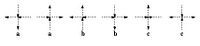
Configurations of the Six vertex model with Boltzmann weights
- Eight-vertex model
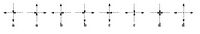
Configurations of the Eight vertex model with Boltzmann weights
- Nineteen-vertex model (Izergin-Korepin model) [4]


References
- ↑ R.J. Baxter, Exactly solved models in statistical mechanics, London, Academic Press, 1982
- ↑ V. Chari and A.N. Pressley, A Guide to Quantum Groups Cambridge University Press, 1994
- ↑ V.E. Korepin et al., Quantum inverse scattering method and correlation functions, New York, Press Syndicate of the University of Cambridge, 1993
- ↑ A. G. Izergin and V. E. Korepin, The inverse scattering method approach to the quantum Shabat-Mikhailov model. Communications in Mathematical Physics, 79, 303 (1981)
 |  |
